How to Reduce Fabric Notebook Startup Time

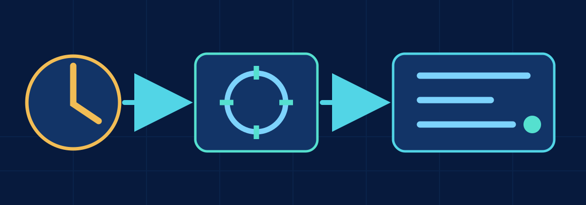
Notebook startup happens before the transformation can usefully process data. For a long batch it may be a small percentage of the run; for many short pipeline notebooks it can dominate end-to-end latency. The right response depends on why Fabric did not take a fast path.

Problem

A notebook’s Spark code completes in under a minute, but the pipeline activity takes much longer. Some runs acquire a session quickly while others wait. Increasing executors will not fix time spent before Spark jobs begin, so first isolate session acquisition from execution.

Why it happens

Fabric starter pools use pre-warmed capacity to reduce session startup when a workload fits their supported configuration. Microsoft describes this as a best-effort optimization: pre-warmed resources are not guaranteed for every run, and fallback to on-demand provisioning can take longer. Custom compute settings, node choices, environment libraries, and networking can affect eligibility and initialization.

Libraries are a frequent source of confusion. Inline installation performs work during an active session. Fabric Environments provide managed dependencies, but publishing mode changes when those dependencies are prepared or installed. Microsoft’s session start insights surfaces whether the session came from a starter pool or on-demand capacity and identifies reasons such as configuration, environment application, libraries, or networking.

A fresh session may also be intentional. Incompatible default Lakehouses, compute configurations, libraries, or identity boundaries prevent sharing. Workloads that need strict isolation should not trade that requirement for startup speed.

Practical recommendations

Measure startup separately. Record the pipeline activity start, session-ready time when available, first Spark job start, and notebook completion. Use the session details or monitoring experience to identify the source and delay reason. Without that split, a slow first data read may be mislabeled as startup.

Prefer the default starter-pool-compatible configuration when it meets the workload. Do not customize node size or Spark properties preemptively. A custom configuration can be correct for a sustained heavy job, but it may exchange a faster execution stage for longer acquisition. Evaluate total duration and reliability.

Move stable, shared dependencies into a governed Fabric Environment rather than running %pip install in every notebook. Choose environment publishing behavior according to development speed, reproducibility, and session needs. Avoid importing heavy packages that the notebook never uses. Package work is part of execution cost even when it is not visible as a Spark stage.

For predictable latency windows, evaluate a custom live pool where supported and justified. Unlike best-effort starter capacity, a live pool keeps dedicated compute warm during its configured window, with an associated capacity tradeoff. Do not keep compute warm all day for a workflow that runs once unless the operational objective warrants it.

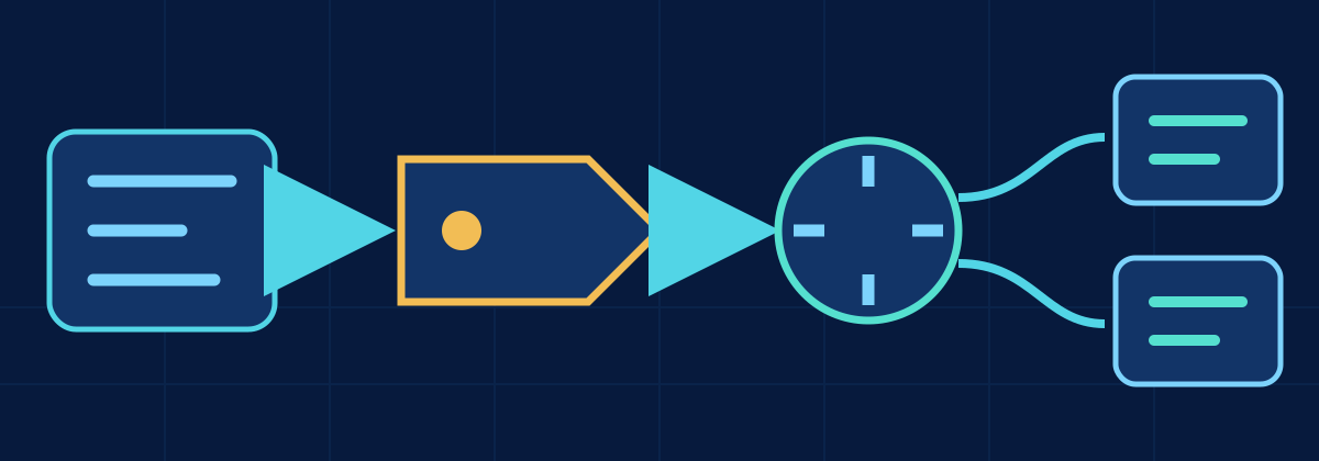
For pipelines containing multiple compatible notebooks, enable high concurrency and use a stable session tag to make reuse possible. Combine that with clear workload boundaries; one memory-heavy notebook can still contend with other workloads in the shared application.

Example measurement pattern

Notebook code cannot measure time before its own process begins, but it can mark the earliest executable point and each subsequent stage. Pair these records with pipeline and Fabric session timestamps.

from datetime import datetime, timezone
from time import perf_counter

notebook_started_at = datetime.now(timezone.utc).isoformat()
clock = perf_counter()

print({"event": "notebook_code_started", "at": notebook_started_at})

orders = (
    spark.read.table("SalesLakehouse.silver.orders")
    .select("order_id", "order_date", "amount")
    .where("order_date >= '2026-10-01'")
)

row_count = orders.count()
print({
    "event": "input_materialized",
    "elapsed_seconds": round(perf_counter() - clock, 3),
    "rows": row_count,
})

If pipeline-to-code time is high but code-to-first-action time is normal, investigate acquisition and environment initialization. If the notebook starts quickly but the first action is slow, inspect table access, file listing, plan creation, and the Spark job instead.

Create a small comparison table across several representative runs:

Run	Session source	Acquisition	First action	Remaining work
Baseline	Starter or reused	measured	measured	measured
Slow run	On-demand or customized	measured	measured	measured

Do not invent target numbers. Establish a baseline for the workspace, capacity, configuration, and time window. Regional demand and concurrent capacity use can change results.

Common mistakes

• Tuning Spark transformations when the delay occurs before the first job.
• Assuming starter-pool startup is guaranteed on every run.
• Adding custom compute or properties without measuring their acquisition cost.
• Installing the same packages inline in every notebook.
• Treating a live pool as free latency reduction without considering capacity use.
• Using unique session tags that prevent related pipeline activities from reusing a session.
• Forcing incompatible workloads together and losing reliability or isolation.
• Measuring one run and presenting it as a stable benchmark.

What to check next

Open the session details for a normal and slow run. Compare session source, delay reason, compute configuration, attached environment, library behavior, networking, capacity conditions, default Lakehouse, and whether a compatible session was already active.

If acquisition is the real issue, simplify configuration, govern dependencies, use session reuse for compatible pipeline activities, or evaluate a live pool for a justified predictable window. If acquisition is normal, move the investigation into the first Spark action and executed plan. Startup tuning ends when code begins; it should not become a convenient explanation for slow reads, shuffles, or Delta writes.