Microsoft Fabric
Pandas vs Polars vs DuckDB vs PySpark in Microsoft Fabric: Speed, Memory and Scale
Compare pandas, Polars, DuckDB, PySpark and Spark SQL in Microsoft Fabric by speed, memory use, data size, Delta support and scale, with measured results from a real Fabric benchmark and practical guidance for choosing the right engine.
On this page
Microsoft Fabric gives you two kinds of notebook and at least five ways to process a table inside them: pandas, Polars, DuckDB and PyArrow in a pure Python notebook, and PySpark, Spark SQL or the pandas API on Spark in a Spark notebook. They are not five syntaxes for the same thing. They are different execution architectures, and the right one depends on how much data you have, how much memory it needs, which Delta Lake features you rely on, and how big the data will be next year.
This guide answers one question: when should you use pandas, Polars, DuckDB or PySpark in Microsoft Fabric? It compares the engines at the architecture level (execution model, speed by data size, memory behaviour, Delta Lake support, supportability and cost) and ends with a decision framework. Along the way it reports what we measured in our own Fabric benchmark on real NYC taxi data, including a notebook orchestration finding that changed how we run Python notebooks in pipelines, and gives you a harness to run on your own capacity. It does not compare syntax; for the API differences between pandas and PySpark, see the Python DataFrames series.
The short version
- Small data that stays small (Microsoft draws the line at roughly 1 GB compressed): a Python notebook with Polars or DuckDB is usually the fastest and simplest choice. pandas is fine for genuinely small frames and is often the right last step.
- 1 GB compressed or more, or data that will grow there: Microsoft recommends the Spark kernel, starting with a single-node 8-vCore session from the starter pool if the data is still modest. PySpark and Spark SQL run on the same engine; pick by team and readability, not by scale.
- Delta-heavy production pipelines (MERGE, UPDATE, DELETE, deletion vectors, OPTIMIZE, VACUUM, Change Data Feed): Fabric Spark. Python engines read Delta well but write only a subset of it.
- Joins, writes and growth decide more than scan speed. A fast local read does not make an engine the right production ETL choice.
- Benchmark your own workload before committing. Microsoft’s benchmark bands below are observations, not thresholds.
What our Fabric benchmark measured
We ran the engines in a Microsoft Fabric pipeline on real NYC Yellow Taxi Parquet data. Three findings are worth knowing before the theory; the full results and method come later.
- On a small dataset, pandas and Polars finished within 0.21 seconds of each other. On dataset S (three Parquet files, 11,198,026 rows, aggregated to 1,240 rows), one run took 2.3387 s of processing in pandas and 2.5467 s in Polars, and both produced identical SHA-256 checksums. It’s a single run on a small input, so it supports “both are fine at this size”, not “pandas is faster”.
- A notebook activity’s duration is not the engine’s processing time. Each standalone Python benchmark activity in the pipeline took 34–38 seconds, while a measured pandas or Polars run on dataset S took 2.3–2.5 seconds of processing. Fabric’s activity duration also covers the notebook session and its lifecycle, so on small data, how you orchestrate notebooks can matter more than which engine you pick.
- One parent notebook beat three separate activities on activity time. A Python runner notebook that called the benchmark notebook once per engine with
notebookutils.notebook.runMultiple()finished in 51 seconds, against 104 seconds summed for three separate notebook activities. No session tags were involved, and it isn’t a controlled wall-clock comparison. The orchestration section explains what it does and doesn’t show.
Two runtimes, not one
Fabric notebooks support a Python kernel, a Spark kernel and a T-SQL kernel. The first two matter here, and they are separate environments with separate versions and lifecycles. Confusing them is the most common source of wrong advice.
| Fabric Python notebook | Fabric Spark notebook (Runtime 2.0) | |
|---|---|---|
| Execution | Single node, no distributed execution | Driver and executors; single node or multi-node |
| Default compute | 2 vCores / 16 GB (1 CU); configurable up to 64 vCores with %%configure |
Starter pool: 8-vCore nodes with autoscale |
| Python version | Kernel you choose: 3.10, 3.11 or 3.12; 3.12 is the default | 3.13, fixed by the runtime |
| Engine versions | Libraries in the Python notebook runtime | Apache Spark 4.1, Java 21, Delta Lake 4.2 |
| Engines | pandas, Polars, DuckDB, PyArrow; delta-rs (deltalake) for Delta |
PySpark, Spark SQL, Scala, SparkR, pandas API on Spark |
| Delta Lake | Read and write through delta-rs and DuckDB; “some Delta Lake features might not be fully supported” | Full feature support |
| Native Execution Engine | No | Yes, when enabled |
Runtime 2.0 is the GA runtime and the default for new workspaces and environment items. Microsoft states explicitly that the Python version inside a Spark runtime is separate from the Python notebook kernel you select: choosing one does not change the other. Python 3.10 reached its announced end of support in October 2026, so new Python notebooks should use 3.11 or 3.12. The Runtime 2.0 vs 1.3 vs 1.2 comparison covers the Spark runtime in detail.
In a Python notebook, Microsoft lists DuckDB, Polars and scikit-learn as preinstalled, ships delta-rs and DuckDB “to support both reading and writing Delta Lake data”, and gives one piece of advice that frames this whole article: if you encounter OOM when loading a large volume of data, try using DuckDB, Polars, or PyArrow dataframe instead of pandas. Library versions in the Python runtime change; the benchmark below records them instead of assuming them.
Execution models first
Before comparing speed, be clear about where the work runs.
- Single nodepandas, Polars, DuckDB, PyArrow
- Notebook processOne Python process on one VM
- Engine in processThreads share one machine's memory
- pandas
- Polars
- DuckDB
- Machine limitUp to 64 vCores in a Fabric Python notebook
- DistributedPySpark, Spark SQL, pandas API on Spark
- DriverPlans the query and schedules tasks
- ExecutorsProcess partitions in parallel
- Partition 1
- Partition 2
- Partition N
- ShuffleMoves rows between executors for joins and aggregates
- Add nodesScale out without rewriting code
- pandas runs eagerly in one Python process. Each step materializes a full DataFrame in memory before the next step starts, and most operations use one core.
- Polars runs on one machine but uses all its cores. Data is held in an Arrow-style columnar format, and the lazy API (
scan_parquet…collect()) lets its optimizer push filters and column selection down to the scan before anything is read. - DuckDB is an embedded analytical database: a vectorized SQL engine inside your Python process, with no server. It queries Parquet files directly (
read_parquet) without first converting them into a DataFrame. - PyArrow is mostly the columnar memory format and I/O layer the others share (Parquet reading and writing, datasets, zero-copy hand-offs). It has compute functions, but it is the plumbing more than the engine you design a pipeline around.
- PySpark and Spark SQL describe a query that a driver plans and executors run in parallel over partitions of the data. Rows move between executors (a shuffle) when a join or aggregation needs them together. Adding nodes adds capacity without changing the code.
Everything else in this article follows from that split: single-node engines start fast and do very little coordination; Spark pays coordination costs that only pay back once the work is big enough to share.
Speed changes with scale
Microsoft’s notebook kernel selection guide reports a clear pattern from end-to-end ELT benchmarks comparing Fabric Spark with the Native Execution Engine against single-machine Python engines (pandas, DuckDB, Polars):
| Compressed data scale | Microsoft-observed pattern |
|---|---|
| Ultra-small, under ~140 MB | Single-machine Python engines (DuckDB, Polars) are faster |
| Small, ~1–2 GB | Python engines still have an advantage; Fabric Spark with the Native Execution Engine becomes competitive as cores per engine increase, particularly for write-heavy operations |
| Small-medium, ~10–13 GB | Fabric Spark with the Native Execution Engine is competitive with or faster than most single-machine engines; single-machine engines can run into OOM at lower vCore counts |
| Medium and above, ~100 GB+ | For most workloads, Fabric Spark with the Native Execution Engine is the fastest and most reliable engine |
These are Microsoft benchmark observations, not limits. The crossover point for your pipeline moves with the operations (scans versus joins versus writes), the number of cores each engine gets, file format and layout, partitioning, compression, memory and cluster configuration.
- Single node fasterUnder ~140 MBDuckDB and Polars avoid distributed overhead
- data growsSingle node ahead~1–2 GBSpark with NEE competitive as cores grow, especially for writes
- data growsCrossover~10–13 GBSpark with NEE competitive or faster; low-core single nodes can OOM
- data growsSpark with NEE ahead~100 GB and aboveFastest and most reliable for most workloads
Why single-node engines win small workloads
For a small table, most of the elapsed time is overhead, not computation. Polars, DuckDB and pandas start executing inside the process that already holds your session: no query has to be split into tasks, no task has to be scheduled on an executor, no rows have to be serialized and shuffled between machines, and no results have to come back to a driver.
Spark pays for all of that on every job: planning and scheduling stages, launching tasks, setting up shuffle files, and coordinating executors. On 100 MB those fixed costs can be most of the run. On 100 GB they are a rounding error, and the parallelism they buy is the whole point.
Session startup is not the whole story
Session startup used to dominate this comparison. In Fabric today, a starter-pool Spark session starts in roughly five seconds, comparable to a Python notebook, and a single-node 8-vCore Spark session from the starter pool starts just as quickly. Custom Spark pools typically take three to five minutes, and Microsoft notes that a Python notebook run that misses its live pool can also take up to three minutes. Measure session start separately from execution; the notebook startup guide shows how to split queue, session and execution time.
Why the Native Execution Engine changes the comparison
The Native Execution Engine (NEE) is why Microsoft’s bands favour Spark as early as they do. It offloads supported Spark operators from the JVM to a vectorized C++ execution path built on Velox and Apache Gluten, with native Parquet and Delta support, while keeping Spark’s optimizer behaviour (adaptive query execution, column pruning, predicate pushdown). It requires no code changes.
What it means for this comparison:
- It narrows the gap single-node engines exploited. Polars and DuckDB are fast partly because they are vectorized, columnar engines. NEE brings the same style of execution to Spark’s operators.
- It helps most where Spark already belongs: computationally intensive queries over Parquet and Delta, joins, aggregations and complex transformations. Microsoft notes the gains are smaller for simple or I/O-bound queries.
- It is not universal. Unsupported operators and features fall back automatically to JVM Spark: structured streaming, and JSON and XML sources, among others. Date comparisons need matching types on both sides. Fallback is visible in
df.explain()and the Spark UI (native operators end inTransformer, or appear asNativeFileScanorVeloxColumnarToRowExec), and Fabric Spark Advisor flags it in the cell output. - It must be enabled. Runtime 1.3 and 2.0 support it; turn it on in the environment’s Acceleration settings or with
spark.native.enabledin%%configure.
Microsoft reports multi-fold improvements in representative benchmark workloads. The specific figure on the runtime page is up to six times faster than open-source Spark on TPC-DS at scale factor 1000 using Delta, which Microsoft translates into roughly 83% compute-cost savings on a fixed-size cluster. Treat that as one benchmark’s ceiling, not a multiplier for your job.
Memory is often the deciding factor
Speed charts make engines look interchangeable until one of them runs out of memory. In practice, memory decides more engine choices than raw speed.
pandas holds every intermediate DataFrame fully in memory, in one process. Compressed Parquet is small on disk; decompressed in-memory columns are larger, and Python-object and string columns can be much larger again. Joins, type conversions and copies multiply the working set. That is why pandas can run out of memory on data whose storage size looks harmless, and why Microsoft’s first OOM advice is to switch away from it.
Polars keeps data in a compact columnar format, uses all cores, and with the lazy API reads only the columns and row groups a query needs. Its streaming engine (collect(engine="streaming") in current versions) processes queries in batches and can handle data that does not fit in memory, but operations that are not implemented in streaming fall back to the in-memory engine, which can bring memory pressure back. It is typically far more memory-efficient than pandas, but the machine is still the limit.
DuckDB executes vectorized SQL directly over files and supports larger-than-memory workloads by spilling to disk: grouping, joins, sorts and window functions can all offload intermediate data to a temporary directory. Its own documentation lists the exceptions: several blocking operators in one query can still raise an out-of-memory error, and some aggregates (such as string_agg) cannot spill.
Spark spreads the working set across executors. Input is split into partitions, each task processes a slice, shuffles distribute intermediate data, and shuffle, sort and aggregation data can spill to disk. Capacity grows by adding workers.
- pandasOne process, eager
- Data grows
- Whole frame in memoryPlus copies from joins and casts
- Memory pressureFar below the node's nominal size
- OOMKernel dies; variables are lost
- Polars and DuckDBOne machine, columnar
- Data grows
- Columnar, pushdownReads only needed columns and row groups
- Batches or spillPolars streaming; DuckDB spills to disk
- Machine limitBigger node, up to 64 vCores, then stop
- SparkDriver plus executors
- Data grows
- PartitionInput split into tasks
- Distribute and shuffleExecutors share the working set; spill to disk
- Add workersSkew, broadcasts and driver collects can still OOM
Spark can still run out of memory
Distributed memory moves the limit; it does not remove it. The classic Spark OOMs are all about concentrating data in one place:
- Driver collection.
collect()andtoPandas()bring the whole result to the driver. - Oversized broadcasts. A broadcast join copies the small side to every executor; broadcasting something that is not small fails on the driver or the executors.
- Skew. One key with a large share of the rows sends that share to one task, however many executors you have.
- Oversized partitions. Too few partitions for the data means each task holds too much.
- Careless caching. Caching large intermediate results takes executor memory from the work that needs it.
- Unbounded state. Long lineage, large window partitions or growing streaming state.
The notebook performance guide and PySpark performance cheat sheet cover how to find and fix these.
Memory comparison
| Engine | Single-node memory limit | Lazy or streaming execution | Spill to disk | Distributed memory |
|---|---|---|---|---|
| pandas | Yes: the whole working set in one process | No: eager, every step materializes | No | No |
| Polars | Yes: one machine | Lazy plans; streaming engine processes in batches, falls back to in-memory for unsupported operations | Not a general mechanism; relies on streaming | No |
| DuckDB | Yes, bounded by its memory limit on one machine | Vectorized pipelines stream through scans | Yes: GROUP BY, JOIN, ORDER BY and window operators; some queries and aggregates can still OOM | No |
| PyArrow | Yes: one machine | Dataset scanning in record batches | No general mechanism | No |
| PySpark, Spark SQL, pandas API on Spark | The driver has its own limit for collects, toPandas() and broadcasts |
Lazy plans, executed per stage | Yes: shuffle, sort and aggregation data | Yes, across executors |
Engines at a glance
| Engine | Execution model | Startup overhead | Memory model | Scale-out | Delta capability in Fabric | Best fit |
|---|---|---|---|---|---|---|
| pandas | Single process, eager, mostly one core | Low | Fully in memory; strings and objects expensive | No | Through delta-rs or Spark, not natively | Small data, final results, Python ecosystem |
| Polars | Single machine, multithreaded, columnar, lazy optimizer | Low | Columnar; pushdown; streaming batches | No | Read; append, overwrite and MERGE; no UPDATE or DELETE | Fast single-node DataFrame ETL |
| DuckDB | Embedded vectorized SQL engine | Low | Vectorized; spills blocking operators | No | Read; INSERT only | SQL over files, ad hoc analytics |
| PyArrow | Columnar format, I/O and compute kernels | Low | Arrow buffers; batch scanning | No | Through deltalake (delta-rs) |
Interchange, Parquet I/O, zero-copy hand-off |
| pandas API on Spark | pandas-style API compiled to Spark | Medium | Distributed | Yes | Full, through Spark | pandas skills on Spark’s engine |
| PySpark DataFrame | Distributed: driver, executors, optional NEE | Medium | Distributed; spills | Yes | Full | Production ETL, large joins, Delta |
| Spark SQL | Same engine as PySpark | Medium | Distributed; spills | Yes | Full | SQL-first teams at any scale |
“Startup overhead” here means per-job coordination as well as session start. A warm Spark session still schedules tasks for every query.
Joins, aggregations and writes
Joins
On a single node, a join is fast if both sides and the result fit comfortably in memory. Polars and DuckDB are excellent at this; pandas is fine while the frames are small. DuckDB can spill a large join to disk; pandas cannot.
In Spark, the join strategy matters more than the input size:
- Broadcast hash join: the small side is copied to every executor and the large side never moves. Spark broadcasts automatically below
spark.sql.autoBroadcastJoinThreshold(10 MB by default in Apache Spark). - Shuffle joins: both sides are repartitioned by the join key so matching rows meet on the same executor. This is what makes large-to-large joins possible, and it is also where most of the cost is.
- Skew: if one key dominates, one task does most of the work. Adaptive query execution, enabled by default since Spark 3.2, can split skewed partitions in sort-merge joins, but it cannot fix a data model where one customer is half the table.
Join shape can matter more than file size. Scanning 100 GB with a selective filter can be cheaper than joining two 5 GB tables on a high-cardinality key, because the join has to move and match every row of both sides. Reduce both sides before the join (filter, project, aggregate to the needed grain), then measure. The PySpark joins cheat sheet has the patterns.
Aggregations
A local vectorized aggregate in Polars or DuckDB is exceptionally fast: no shuffle, every core working on one shared memory space. Spark aggregates in two phases, partial aggregation on each executor and then a shuffle to combine the partials, which adds overhead on small data and scales on large data.
Single-node aggregation stops being the better choice when the hash table no longer fits (high-cardinality group keys), when the input is too large to scan in acceptable time on one machine’s cores, when several users or jobs share the same capacity, or when the aggregate is one step in a pipeline whose writes and joins are the real bottleneck.
Writes matter more than benchmarks suggest
Benchmarks often measure reads, because reads are easy to compare. Production pipelines also write, and writes separate the engines more than scans do:
- Parquet writes are well supported everywhere. Spark writes many files in parallel (one or more per task); single-node engines usually write one or a few. Neither is wrong, but file count and size affect every later read; see Delta table maintenance for the small-files problem.
- Delta writes are where the engines differ most: transaction semantics, MERGE, UPDATE and DELETE, deletion vectors, checkpoints and maintenance. The next section has the details.
- MERGE at scale is a join plus a rewrite of the affected files. Spark with deletion vectors handles it as merge-on-read; the Delta MERGE performance patterns apply there.
- Concurrent writers need conflict detection. Spark and delta-rs implement optimistic concurrency control; a DuckDB INSERT does not detect conflicts.
A fast local scan does not make an engine the best production ETL choice. The engine has to finish the write correctly, transactionally, and in a layout the next reader can use.
Delta Lake compatibility
This is the deciding factor for many Fabric pipelines, because Lakehouse tables are Delta tables. The table below summarizes Microsoft’s feature matrix, which reflects direct testing against Fabric Spark Runtime 1.3 and 2.0 as of June 2026. The open-source Python Delta ecosystem releases often; check each project’s release notes before relying on a feature.
| Delta feature | Fabric Spark | delta-rs (deltalake) |
DuckDB | Polars |
|---|---|---|---|---|
| Read Delta tables | Yes | Yes | Yes | Yes |
| Append and overwrite | Yes | Yes | INSERT only, no schema evolution | Yes |
| MERGE | Yes | Yes | No | Yes |
| UPDATE and DELETE | Yes | Yes | No | No |
| Write deletion vectors | Yes | No | No | No |
| Read deletion vectors | Yes | No | Yes | Yes |
| OPTIMIZE | Yes | Yes | No (use delta-rs) | No (use delta-rs) |
| VACUUM | Yes | VACUUM LITE only | No | No |
| Write Change Data Feed | Yes | No | No | No |
| Liquid Clustering writes | Yes | No | No | No |
| Checkpoints | Every 10 commits by default | Configurable, default 100 | INSERT writes none | Configurable, default 100 |
The consequences Microsoft calls out:
- Deletion vectors are enabled by default for new tables starting in Runtime 2.0, and no Python engine can write them. Writing with a Python engine to a table that has deletion vectors enabled causes compatibility errors.
- Cross-engine pipelines need version pinning. If Polars or DuckDB reads and delta-rs writes, both sides must pin the table version to keep read-then-write isolation.
- Tables written only by Python engines accumulate small files and long transaction logs unless you run delta-rs maintenance yourself; DuckDB INSERT never writes checkpoints.
- Row tracking metadata (
row_id,row_commit_version) is only readable in Spark, so CDC or deduplication logic that depends on it must read with Spark.
Microsoft’s own recommendation is to treat Python engines as a complement to Spark for lightweight reads, local development and simple appends, rather than a general-purpose replacement. For the Delta model itself, see Delta tables for SQL Server engineers.
Supportability
This is the architect’s question that speed charts never answer: who fixes it when it breaks?
Fabric Spark is Microsoft’s own fork of Apache Spark. Microsoft maintains and ships the runtime, supports Spark and Delta internals end to end, including the Native Execution Engine, and accepts support tickets for Spark behaviour, query plans, memory issues and engine bugs. Runtime updates bring performance improvements to existing code.
DuckDB and Polars are open-source engines that Fabric makes available. Microsoft does not maintain forks of them. Its support covers the OneLake integrations shipped in the Fabric runtime, such as authentication and file system access. An engine bug, a performance regression or an API change between library versions goes to the open-source community. Microsoft also notes that API changes between versions can require refactoring, that neither engine has a live monitoring equivalent to the Spark UI, and that a full ELT stack built on them usually stitches several libraries together (DuckDB for transformation, delta-rs for writes and maintenance) whose versions you then keep compatible.
None of that makes them a bad choice. It makes them a choice whose operational risk you own. For a notebook an analyst runs on demand, that is usually fine. For the pipeline that feeds a finance close, it deserves an explicit decision.
Cost and concurrency
“Spark always costs more” is a myth, and so is the reverse. Fabric bills compute as capacity units over time, so for a given configuration:
Cost = resources reserved × elapsed time.
Microsoft’s selection guide gives the reference points:
| Configuration | vCores | Capacity units while running |
|---|---|---|
| Python notebook, default | 2 | 1 CU |
| Python notebook, largest | 64 | 32 CU |
| Spark, 4-vCore single node (custom pool, slower start) | 4 | 2 CU |
| Spark, 8-vCore single node (starter pool) | 8 | 4 CU |
| Spark starter pool, after proactive scale-up | 8-core workers | 8 CU minimum |
Two consequences:
- On small work, a 2-vCore Python notebook that finishes in the same time as Spark uses a fraction of the capacity. The single-node 8-vCore Spark configuration exists to narrow that gap while keeping Spark’s features.
- On large work, an engine that finishes several times faster on more cores can consume less in total than a smaller engine running much longer, or one that fails and reruns.
Real capacity accounting has more nuance (smoothing, bursting, background versus interactive operations); see Fabric capacity explained before making CU promises to a finance team.
Concurrency changes the picture again. Five analysts each running a 64-vCore Python notebook reserve five large nodes; Spark’s high-concurrency mode lets compatible notebooks share one session, and Spark pools isolate workloads. Microsoft lists high concurrency and FAIR or FIFO job scheduling among the reasons to choose the Spark kernel. When many jobs share a capacity, choose the engine for the capacity, not only for one job.
Spark first, pandas last
The most expensive single line in many Fabric notebooks is this one:
pdf = spark_df.toPandas() # on a large DataFrame: every row moves to the drivertoPandas() collects the entire Spark DataFrame into the driver’s memory and converts it to pandas. On a large table, that turns a distributed job into a single-machine one at the worst possible moment, and the driver runs out of memory long before the executors would have. Microsoft’s guidance is direct: only use it for small to medium result sets; filter, aggregate or sample in Spark first.
- 2 TBLakehouse tablesStay in Spark
- SparkFilter and projectPredicates pushed down; only needed columns read
- SparkAggregateReduce to the grain the analysis needs
- 20 MBSmall resultFits comfortably in driver memory
- toPandas()pandasPlotting, machine learning, Python libraries
from pyspark.sql import functions as F

monthly = (spark.read.table("sales_orders")
           .where(F.col("order_date") >= "2026-01-01")
           .groupBy("region", F.trunc("order_date", "month").alias("month"))
           .agg(F.sum("amount").alias("revenue")))

pdf = monthly.toPandas() # a few hundred rows, not two terabytesThe same rule applies in the other direction: do not load a large file into pandas in a Python notebook “to look at it”. Use Polars or DuckDB to reduce it, then convert the small result if a library needs pandas.
Where each engine shines
pandas: the right last mile
pandas is not the villain of this article. It remains excellent for small data, for final result sets, for data science work, and above all for ecosystem compatibility: plotting libraries, statistics and machine learning packages, and countless downstream tools expect a pandas DataFrame. pandas is often the right last mile, not the right first mile for huge data. Its limits are single-process execution and in-memory everything, not quality.
Polars: fast single-node DataFrames
Polars is attractive for notebook exploration, file-to-file transformations, medium-size datasets that fit one machine, and high-performance single-node ETL, with a DataFrame API that feels familiar. Use the lazy API (scan_parquet instead of read_parquet) so the optimizer can prune columns and row groups before reading.
import polars as pl

top_customers = (pl.scan_parquet("/lakehouse/default/Files/raw/orders/*.parquet")
                 .filter(pl.col("status") == "shipped")
                 .group_by("customer_id")
                 .agg(pl.col("amount").sum().alias("revenue"))
                 .sort("revenue", descending=True)
                 .head(100)
.collect())It is not “mini Spark”. It does not distribute, it has no cluster to grow into, and when the data outgrows the largest node, the code has to move.
DuckDB: SQL over files
DuckDB fits SQL-first analysis: scanning Parquet, joining files to files, ad hoc exploration and embedded analytical processing inside a Python notebook, without loading anything into a DataFrame first. In a Python notebook with a default lakehouse attached, Lakehouse files are available under /lakehouse/default/Files/:
import duckdb

duckdb.sql("""
    SELECT region, date_trunc('month', order_date) AS month, sum(amount) AS revenue
    FROM read_parquet('/lakehouse/default/Files/raw/orders/*.parquet')
    WHERE status = 'shipped'
    GROUP BY ALL
    ORDER BY ALL
""").df() # convert the small result for pandas-based toolsFor Lakehouse tables, start from the snippet the notebook generates (drag the table onto the canvas or use Load data), which uses the Delta libraries shipped with the runtime. DuckDB’s Delta writes are INSERT-only, so use delta-rs for anything else.
PySpark and Spark SQL: one engine, two languages
PySpark and Spark SQL compile to the same plans and run on the same Spark compute, including the Native Execution Engine. Microsoft describes the Spark kernel’s languages (PySpark, Spark SQL, Scala, SparkR) as “all backed by the same Spark compute”. Spark SQL does not mean smaller scale than PySpark.
Choose by expression style and team skill:
- Spark SQL for set-based transformations a SQL team will read and review, and for logic that maps naturally to
SELECT … JOIN … GROUP BY. - PySpark for programmatic pipelines: parameterized column lists, reusable functions, dynamic schemas and unit-testable transformations (see PySpark unit testing with pytest).
Mixing them in one notebook is normal: spark.sql(...) returns a DataFrame and createOrReplaceTempView exposes one to SQL.
pandas API on Spark: familiar syntax, distributed engine
The pandas API on Spark (import pyspark.pandas as ps) gives pandas-style syntax on top of Spark’s distributed engine. It makes sense for teams with strong pandas skills, for moving existing pandas logic to larger data, and as a migration aid. For heavy production engineering, native PySpark or Spark SQL is usually clearer: the mapping from pandas semantics (row order, index alignment) to a distributed engine can hide expensive operations, and plans, joins and partitioning are easier to reason about in the native APIs. It is a legitimate option, not a shortcut around understanding Spark.
Design for tomorrow’s volume, not today’s sample
Engine decisions are usually made on today’s data:
| Daily volume | What a single-node pipeline feels like | |
|---|---|---|
| Today | 700 MB | Fast, cheap, simple |
| In six months | 15 GB | Larger node, longer runs, occasional OOM |
| In two years | 200 GB | Rewrite |
The rewrite is the expensive part: different APIs, different Delta write paths, different tests, different monitoring, and a migration done under pressure because the job already fails. Microsoft makes the same point in its selection guide: migrating code when data exceeds a non-distributed engine’s limits is costly, and starting with Spark on a single-node configuration lets you scale out to multiple nodes without rewriting the pipeline.
So ask two questions, not one: how big is the data? and how big will it be within the life of this pipeline? If the honest answer to the second is “large, or unknown”, start in Spark, even if a single-node engine wins today’s benchmark.
A decision framework by data size
Microsoft’s guidance is the anchor: use the Python kernel for data under approximately 1 GB compressed when single-machine performance matters most, and the Spark kernel at 1 GB compressed or more, or when you expect data to grow to that scale. The bands below are my own working heuristics around that line.
| Compressed input | Starting point | Why |
|---|---|---|
| Under ~1 GB, stable | Polars or DuckDB in a Python notebook; pandas for genuinely small frames | Lowest overhead; Microsoft’s Python-kernel range |
| Under ~1 GB, growing | Spark, single-node 8-vCore from the starter pool | Same fast start, no rewrite later |
| ~1–10 GB | Benchmark both; default to Spark for production pipelines | Microsoft recommends Spark from 1 GB; single-node engines can still win reads and interactive work |
| ~10–100 GB | PySpark or Spark SQL for production pipelines | Microsoft’s crossover band; joins, writes and OOM risk favour Spark |
| ~100 GB and above | PySpark or Spark SQL with the Native Execution Engine | Microsoft observes Spark with NEE fastest and most reliable for most workloads |
Whatever the size, two conditions push toward Spark on their own: Delta features Python engines cannot write (deletion vectors, MERGE-heavy patterns with DuckDB, UPDATE and DELETE with Polars, Change Data Feed, Liquid Clustering), and large joins or writes.
Decision guidance by workload
Javi Builds decision guidance (not a Microsoft requirement). “Strong fit”: a sensible default. “Possible”: works, but not the obvious choice. “Benchmark first”: the answer depends on your data and capacity. “Usually avoid”: a poor fit for that architecture.
| Workload | pandas | Polars | DuckDB | PySpark | Spark SQL |
|---|---|---|---|---|---|
| 100 MB filter | Possible | Strong fit | Strong fit | Possible | Possible |
| 1 GB aggregation | Benchmark first | Strong fit | Strong fit | Possible | Possible |
| 10 GB join | Usually avoid | Benchmark first | Benchmark first | Strong fit | Strong fit |
| 100 GB transformation | Usually avoid | Usually avoid | Usually avoid | Strong fit | Strong fit |
| Large Delta MERGE | Usually avoid | Usually avoid | Usually avoid | Strong fit | Strong fit |
| Interactive exploration of small data | Strong fit | Strong fit | Strong fit | Possible | Possible |
| Repeated SQL analytics on modest files | Usually avoid | Possible | Strong fit | Possible | Strong fit |
| Large distributed ETL | Usually avoid | Usually avoid | Usually avoid | Strong fit | Strong fit |
Decision tree
- Size the workloadCompressed input today and over the pipeline's life
- Fits one node, and stays?The first three branches assume yes
- SQLDuckDBSQL over Parquet and Delta reads
- DataFramesPolarsLazy, multithreaded transforms
- resultspandasSmall results for the Python ecosystem
- growingPySpark or Spark SQLStart single-node 8-vCore; scale out later
- DeltaSpark with NEEMERGE, deletion vectors, OPTIMIZE, large joins
Real Fabric benchmark
Microsoft’s guidance and this benchmark are different kinds of evidence. The benchmark bands quoted earlier are a documented reference from Microsoft. The Javi Builds benchmark is an observed experiment: one realistic workload in one Fabric workspace (ws_fabric_engine_benchmark), orchestrated by one pipeline (pl_fabric_engine_benchmark), with every published number traced to a run. It sits next to Microsoft’s bands; it does not replace them.
The results below come from a pilot: the pipeline ran all six engine configurations (pandas, Polars, DuckDB, PySpark, Spark SQL and PySpark with the Native Execution Engine), but the engine-level timings published so far are single runs for pandas and Polars on one dataset size. The controlled, repeated runs described under Method are the next step. Where a value was not measured, this section says so instead of estimating it.
Three performance dimensions, never one ranking
A Fabric benchmark produces three kinds of duration. They answer different questions, and adding or ranking them together gives a misleading result.
| Dimension | What it measures | Where it comes from | Example from this experiment |
|---|---|---|---|
| Engine processing time | The engine’s work from read to write, stage by stage | Timers inside the benchmark notebook | pandas 2.3387 s, Polars 2.5467 s on dataset S (one run) |
| Notebook activity duration | One pipeline activity end to end: notebook session, parameters, imports, the engine work and the activity lifecycle | Duration column in the pipeline’s Output tab | Standalone Polars activity: 34 s |
| Pipeline wall-clock time | First activity start to last activity end, including parallel branches and waits | The pipeline run, or derived from the activity table | About 7 min 54 s for the latest run |
The gap between the first two rows is the main lesson for small data: a standalone Python benchmark activity took 34–38 seconds, while the processing it exists to measure took about 2.5 seconds in a measured run. An engine comparison has to use the first row. A pipeline design comparison uses the second and third.
Dataset
The input is real public data: the NYC Taxi & Limousine Commission Yellow Taxi trip records for 2025, in the official monthly Parquet files, plus the official taxi-zone lookup. The twelve 2025 files total about 840 MB compressed and 49.4 million rows, with identical column types in every month.
| Level | Input | Status |
|---|---|---|
| XS | One month of 2025 | Used by the Spark activities in the pilot |
| S | Three monthly files | Verified: 11,198,026 raw records, 1,240 aggregated rows |
| M | Twelve months | Planned |
| L, XL | Repeated copies of the twelve months, built on Spark to roughly 10 GB and 100 GB | Planned |
The larger levels are labelled for what they are: repeated/scaled copies of real TLC data for performance testing. Each copy carries a benchmark_replica_id, so the schema and value distributions are real but the trips are not unique.
Workload
Every engine runs the same logical pipeline on the same staged files, from Parquet to Parquet, in six timed stages: read, transform, aggregate, join, sort, write.
- same filesStaged TLC ParquetFingerprinted by file name and size
- 8 columnsProject and filterPositive distance and amount, dropoff after pickup
- zone, paymentAggregateTrips, revenue, tips, average fare, distance, duration
- zone lookupJoin and sortLeft join on pickup zone, revenue descending
- writeOne Parquet fileThen validated against every other engine
- Transform: keep trips with a positive distance and total amount and a dropoff after the pickup, then derive the trip duration in minutes.
- Aggregate: group by pickup zone and payment type (1,240 groups on dataset S) and compute trip count, revenue, tips, average fare, average distance and average duration.
- Join: a left join from the aggregate to the taxi-zone lookup on the pickup zone ID, so groups with an unknown zone are kept with empty zone names rather than dropped.
- Sort and write: revenue descending with deterministic tie-breakers, written as one Parquet file.
Results: pandas and Polars on dataset S
| Stage | pandas | Polars |
|---|---|---|
| Read | 1.1506 s | 1.0510 s |
| Transform | 0.2203 s | 0.2103 s |
| Aggregate | 0.7495 s | 1.0863 s |
| Join | 0.0752 s | 0.0663 s |
| Sort | 0.0054 s | 0.0065 s |
| Write | 0.1377 s | 0.1263 s |
| Total | 2.3387 s | 2.5467 s |
What the numbers support:
- Both engines produced the same answer. 1,240 output rows, total revenue of $287,431,793.68, total tips of $31,903,631.09, and identical SHA-256 checksums.
- Reading and aggregating are the work. Read plus aggregate is 81% of the pandas total and 84% of the Polars total. Once 11.2 million rows become 1,240 groups, the join, sort and write cost almost nothing.
- Polars was not run in its best mode here. Stage timings require each stage to finish before the next starts, so Polars had to materialize every intermediate result instead of letting its lazy optimizer plan the whole pipeline at once. The aggregate stage, where the gap is largest, is exactly where a fused lazy plan would differ. An end-to-end lazy run is a separate measurement, and the next one to take.
- At this size, the engine choice is a few hundred milliseconds. That’s the same conclusion as Microsoft’s smallest band: on small data, single-node engines are all fast, and overhead elsewhere dominates.
Other engines in the pilot
DuckDB, PySpark, Spark SQL and PySpark with the Native Execution Engine all ran successfully as pipeline activities. Their engine processing times on dataset S are not published, because the measurements that would make them comparable (the same dataset, repeated runs, cross-validated output) do not exist yet. Their pipeline activity durations are in the orchestration section, and they are not engine timings: a Spark activity’s duration includes acquiring a Spark session, and the Spark activities processed dataset XS.
Method
What the pilot did. pandas, Polars and DuckDB ran in a Fabric Python notebook (nb_fabric_engine_python), parameterized by engine, dataset_scale and run_count; PySpark, Spark SQL and PySpark with the Native Execution Engine ran in Spark notebooks. A pipeline staged the data, then ran the engines. Each engine’s notebook timed the six stages and wrote a checksum of its output.
What the controlled runs will do. For each engine and dataset size:
- Repetitions: one first run in a fresh session, then at least five subsequent runs, reported as the median with minimum and maximum. Every run is kept, including failures. Five is the minimum for a published performance claim; fewer runs cannot separate small differences from noise.
- Timing: both a stage-by-stage run (to show where time goes) and an end-to-end run (each engine’s own best plan, including the write). Spark timings always end in an action, so a lazy plan is never mistaken for work done.
- Isolation: one engine per freshly restarted Python kernel, so each memory figure is its own; a fresh session per Spark configuration; children of a runner notebook run one at a time while being timed.
- Session start recorded separately from execution, and never included in engine processing time.
- Environment recorded from the session at run time: capacity, Python notebook vCores, Spark pool and node size, runtime, library versions, and whether native execution actually appeared in the query plan.
Reading the results: what moves the numbers
- Python versus Spark compute. A Python notebook runs on one node, 2 vCores and 16 GB by default; a Spark notebook runs a driver and executors from a pool. Comparing them compares hardware as well as engines, so record both and repeat with matched cores where you can.
- Native Execution Engine. NEE accelerates supported Spark operators and falls back silently for others. Check the plan (
*Transformer,NativeFileScan) rather than trusting an activity name. - Cold versus warm notebook execution. A Python notebook that misses Fabric’s live pool can take up to three minutes to start; one that hits it starts in seconds. That variation lands in activity duration, not in engine processing time. In this pilot, the first successful runner run took 1 min 21 s, later runs 50 and 51 s.
- Caching and memory. Re-reading the same files benefits from the operating system’s page cache, engine-level metadata caches, and Spark’s intelligent cache. A first run and a fifth run measure different things; report both.
- Lazy versus eager. pandas does each step as it is called. Polars’ lazy API and Spark plan first and execute on collect or an action. Stage timing forces execution at every stage and penalizes lazy engines; end-to-end timing does not.
- Spark action materialization.
df.filter(...)returns instantly because nothing ran. A Spark timing that does not end incount(),collect()or a write measures planning, not processing. - Shared resource contention. Activities on the same capacity, children of one runner notebook, and other users’ jobs share resources. Two activities that overlap in time can slow each other down.
- Repeated runs and statistical variability. Spark activity durations in this pilot varied by more than a minute between runs of the same notebook. Single runs describe one moment; medians over at least five runs describe the engine.
Validation
Each run produces a result signature. The row count, the total trip count and a hash of every group with its zone names and trip count must match exactly across engines. Money totals must agree to the cent and averages to a relative 1e-9, because engines add floating-point numbers in different orders. A run that disagrees is marked VALIDATION_FAILED and its timing is excluded. Failures are kept as results: an engine that runs out of memory, errors, or is skipped by the pandas safety limit is reported as such, not silently dropped.
In the pilot, pandas and Polars matched on every check: row count, revenue, tips and the SHA-256 checksum of the full output.
Evidence
| Evidence | Value |
|---|---|
| Dataset | NYC TLC Yellow Taxi trip records, 2025; dataset S: three Parquet files |
| Rows | 11,198,026 raw records; 1,240 aggregated rows |
| Output totals | Revenue $287,431,793.68; tips $31,903,631.09 |
| Engines with published processing times | pandas, Polars |
| Engines executed in the pipeline | pandas, Polars, DuckDB, PySpark, Spark SQL, PySpark with NEE |
| Repetitions | 1 run per engine (pilot) |
| Validation | Identical SHA-256 checksums for pandas and Polars |
| Workspace and pipeline | ws_fabric_engine_benchmark, pl_fabric_engine_benchmark |
| Pipeline runs shown | 11 November 2026 |
| Fabric capacity | Not recorded in the published evidence |
| Python notebook compute | Not recorded in the published evidence |
| Spark runtime and pool | Not recorded in the published evidence |
| Native execution | A separate PySpark NEE activity ran; plan-level evidence not yet published |
A Delta Lake benchmark (read, append, MERGE, UPDATE, DELETE) is planned as a separate experiment. The engines do not support the same Delta operations, so mixing Delta into this comparison would make it unfair.
Optimizing Microsoft Fabric Notebook Orchestration Without Session Tags
The most useful finding of the pilot was not about engines. It was about how the pipeline started the Python notebooks.
The original design: one pipeline activity per engine
The first version of the pipeline ran a setup notebook, then one Notebook activity per engine, one after another: Benchmark_Pandas, Benchmark_Polars and Benchmark_DuckDB (each calling nb_fabric_engine_python with a different engine parameter), then the three Spark activities.
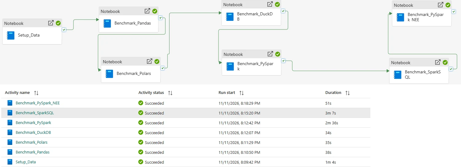
Each Python activity took 34–38 seconds. A measured pandas or Polars run on dataset S does about 2.5 seconds of engine work, so on small data most of an activity like this is the cost of running a notebook as a pipeline activity, paid three times.
The change: one runner notebook calling a child notebook per engine
We added a parent Python notebook, nb_fabric_benchmark_runner. It calls the existing benchmark notebook once per engine with notebookutils.notebook.runMultiple(), passing a different engine argument each time, and fails if any child fails. In the pipeline, it runs on its own branch after Setup_Data, and the three standalone Python activities are set to Inactive.
- Separate activitiesOriginal pipeline
- Setup_Data
- Benchmark_Pandas35 s activity
- Benchmark_Polars34 s activity
- Benchmark_DuckDB35 s activity
- Spark activitiesStart after DuckDB, about 110 s after setup
- Runner notebookLatest pipeline
- Setup_Data
- benchmark_runner51 s activity; Python notebook, runMultiple()
- pandas child
- Polars child
- DuckDB child
- in parallelSpark activitiesStart 2 s after setup
A runner of this shape is short. The values below are illustrative, not a copy of our notebook; dataset_scale and run_count come from the runner’s parameter cell:
# Fabric Python notebook (the runner). Children must also be Python notebooks.
from time import perf_counter
from notebookutils.common.exceptions import RunMultipleFailedException

dag = {
    "activities": [
        {
            "name": f"benchmark_{engine}",
            "path": "nb_fabric_engine_python",           # the existing benchmark notebook
            "args": {"engine": engine, "dataset_scale": dataset_scale, "run_count": run_count},
            "timeoutPerCellInSeconds": 1800,              # default is 90 seconds per cell
        }
        for engine in ["pandas", "polars", "duckdb"]
    ],
    "concurrency": 1,  # run children one at a time while they are being timed
}

notebookutils.notebook.validateDAG(dag)  # catches structural and compute-type errors early
start = perf_counter()
try:
    results = notebookutils.notebook.runMultiple(dag)
except RunMultipleFailedException as error:
    results = error.result
print(f"Runner wall time: {perf_counter() - start:.2f} s")

failures = {name: str(info["exception"]) for name, info in results.items() if info["exception"] is not None}
if failures:
raise RuntimeError(f"Benchmark failures: {failures}")Two settings matter for benchmarks. concurrency defaults to three times the node’s CPU cores, so without it the children run at the same time and their engine timings include each other’s load. timeoutPerCellInSeconds defaults to 90 seconds, which a larger dataset will exceed.
What the pipeline runs showed
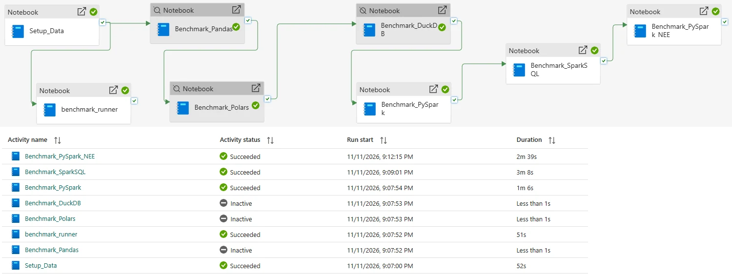
Three pipeline runs on 11 November 2026 trace the change. Run B is a transition run in which the runner and the standalone activities both ran, at the same time, so its activity durations were measured under shared load.
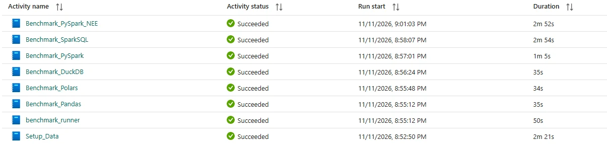
| Run A: separate activities | Run B: both | Run C: runner only | |
|---|---|---|---|
| Standalone pandas, Polars, DuckDB | 38 s, 35 s, 34 s | 35 s, 34 s, 35 s | Inactive |
| Sum of the three | 107 s | 104 s | — |
benchmark_runner |
Not in the pipeline | 50 s, alongside the standalone activities | 51 s |
| Spark chain starts after setup ends | About 116 s later | About 110 s later | About 2 s later |
| PySpark, Spark SQL, PySpark NEE | 2m 36s, 3m 7s, 51s | 1m 5s, 2m 54s, 2m 52s | 1m 6s, 3m 8s, 2m 39s |
| Pipeline wall-clock (derived) | About 9 min 38 s | About 11 min 5 s | About 7 min 54 s |
The derived rows are computed from the activity table’s start times and whole-second durations, so they are accurate to a few seconds; they are not separately measured pipeline durations.
What the 51% means, and what it doesn’t
The runner’s 51 seconds is about 51% less than the sum of the three separate activity durations (104 seconds). That is the only comparison these runs support directly, and three qualifications apply:
- It is not a pipeline wall-clock comparison. In the original pipeline the three activities ran one after another, so their sum is close to the time they occupied (107 seconds from Pandas start to DuckDB end in run B). A pipeline that ran the three activities in parallel would take roughly as long as the slowest one, not 104 seconds. We did not run that variant, so we cannot say the runner beats it.
- It does not isolate runtime reuse. Child notebooks called with
runMultiple()run inside the caller’s session and share its compute; Microsoft documents that the API “uses a multithreaded implementation within a Spark session, which means referenced notebook runs share compute resources.” Starting one notebook session instead of three is the plausible reason the runner is shorter, but we did not record session start, child durations or child overlap separately, so the share of the saving that comes from avoided session start-up is unmeasured. - It compares different runs under different conditions. Run B’s standalone durations were measured while the runner was also running, and run C’s runner ran alongside PySpark. Two runs on one evening are not a distribution.
The pipeline-level effect is easier to see, and it is not the 51%. In runs A and B the Spark activities waited about 110–116 seconds for the Python chain; in run C they started 2 seconds after setup, because the Python benchmarks moved to a parallel branch. The Spark activities’ combined duration was similar in all three runs (394, 411 and 413 seconds), so the shorter latest pipeline mostly reflects that removed wait, not faster engines. Individual Spark activities varied far more than the runner did: the NEE activity took 51 seconds in one run and over 2.5 minutes in the other two.
Parent and child compute types must match
The first runner was a Spark notebook. Validating its DAG failed before any child ran:
ChildNotebook compute type JupyterCompute does not match to main notebook compute type SparkComputeJupyterCompute is the Python notebook (the child, nb_fabric_engine_python); SparkCompute is the Spark notebook that called it. A referenced notebook runs on the caller’s compute, and Fabric checks that the parent’s and the child’s compute types match before it runs anything. The fix was to make the runner a Python notebook, which Microsoft documents as supported: Python notebooks can reference-run other Python notebooks with notebookutils.notebook.run() or runMultiple(). Call validateDAG() first and this error surfaces in a second, not after a long run.
The rule generalizes: group child notebooks by compute type. Python children under a Python runner, Spark children under a Spark runner (or as separate pipeline activities). The Spark engines in this pipeline stayed as their own activities for that reason.
When notebook-to-notebook orchestration helps
- Many short notebooks where session start is a large share of each activity, like the 34–38 second Python activities here doing 2.5 seconds of work.
- The same notebook run with different parameters (an engine, a table, a date): one parameterized child and a DAG of arguments.
- Children with the same compute type and default lakehouse. A reference run is blocked if the child declares a different default lakehouse from the parent.
- When one pipeline activity is the right unit of monitoring and retry, with the runner raising an error if any child failed.
When it may not help
- Long-running children. If each child runs for twenty minutes, a few seconds of session start are noise, and you lose per-activity visibility in the pipeline for nothing.
- Children that compete for one node. Children share the runner’s compute. On a default 2-vCore Python notebook, three memory-hungry children running at once can be slower than three separate activities, or run out of memory together.
- Mixed compute types or sizes. Spark and Python children cannot share a runner, and every child gets the runner’s node size.
- Per-activity control in the pipeline. Separate activities give each notebook its own retry policy, timeout, dependency conditions and status in the Monitoring hub. A runner moves that logic into Python.
- Spark notebooks that could share a session another way. For Spark activities, high concurrency mode for pipelines and session tags are the documented session-sharing mechanism; they were not used here and are a separate experiment.
How to measure the difference
To turn this observation into a controlled result, run the same pipeline in each design, on the same dataset and capacity:
- Variants: separate sequential activities, separate parallel activities, and one runner with
concurrency: 1(and, separately, an unrestrictedconcurrency). - Runs: at least five per variant, alternating the order of variants so time-of-day effects spread evenly.
- Record three numbers per run: each activity’s duration from the Output tab, the pipeline wall-clock time, and inside the runner, each child’s duration (time each
runMultipleactivity, or have each child return its timings withnotebookutils.notebook.exit()). - Record session start for each variant from the Monitoring hub, so session reuse can be measured instead of inferred.
- Compare medians with minimum and maximum, per metric. Never combine activity time, wall-clock time and engine processing time into one score.
The notebook startup guide shows how to separate queue, session and execution time, and monitoring Fabric pipelines and notebooks covers where each duration is reported. For passing engine-style arguments, see Fabric notebook parameters; for the wider trade-off, pipelines vs notebooks in Fabric.
Benchmark this on your own Fabric capacity
Microsoft’s bands tell you where to look. Your own numbers tell you what to choose. The method below compares Polars, DuckDB and pandas in a Python notebook with PySpark and Spark SQL in a Spark notebook, on the same files and the same workload.
What to test
Generate (or copy) the same input at several sizes, for example ~100 MB, ~1 GB and ~10 GB compressed, and larger if your capacity allows. Run one realistic pipeline, not a single operation:
- read Parquet;
- filter;
- join to a dimension;
- group and aggregate;
- sort;
- write the result.
Do not benchmark only a count(): Spark can answer some counts from metadata, Polars and DuckDB can skip most of the data, and none of it says anything about joins or writes.
What to record
- Session start time, separately from execution (notebook status bar or Monitoring hub).
- Execution time for the whole pipeline, including the write.
- Peak process memory for single-node engines; executor memory and spill for Spark (see the caveats below).
- Output: file count, and a checksum (row count and totals) proving every engine produced the same result.
- Success, error or OOM, per run.
- Repeatability: at least five runs per engine and size, reported as the median with minimum and maximum.
- Activity duration and pipeline wall-clock time, separately from engine processing time, if the benchmark runs in a pipeline.
- Environment: capacity SKU, Python notebook vCores or Spark pool and node size, Spark runtime, whether NEE was enabled, library versions, source format and compressed input size.
Fair benchmarking rules
- Same source files, same columns and filters, same output semantics, verified by checksum.
- Separate the first run in a session from subsequent runs; caches (DuckDB’s, Spark’s intelligent cache, the OS) favour repeated reads, and a truly cold read is hard to guarantee.
- Give engines comparable cores where you can: a 2-vCore Python notebook against an 8-vCore Spark node is a comparison of hardware, not engines. Repeat with the Python notebook at 8 vCores (
%%configure). - Measure startup separately from execution.
- Run each case several times and report the median, with every run kept. Do not cherry-pick the fastest run.
- Include pandas only at sizes it can survive, and never benchmark by deliberately crashing a shared capacity.
Python notebook harness: Polars, DuckDB, pandas
Run this in a Python notebook with a default lakehouse attached. It generates synthetic orders and customers with DuckDB, then runs the same workload five times per engine, sampling peak process memory and writing one JSON line per run. pandas is skipped above PANDAS_MAX_BYTES, so the benchmark never deliberately exhausts memory. Increase ORDER_ROWS and change SIZE_LABEL for each size, and record the compressed size it prints rather than the row count. Library APIs move between versions (DuckDB 2.0 removed fetchone() from relations, for example), which is why the harness records versions and sticks to long-standing calls.
# Fabric Python notebook (pure Python kernel), default lakehouse attached.
# Cell 1: configuration and synthetic data. Same files are read by every engine.
import json, os, platform, statistics, threading, time
from datetime import date

BASE = os.environ.get("BENCH_BASE", "/lakehouse/default/Files/engine-bench")
SIZE_LABEL = "s1"                 # one folder per dataset size: s1, s2, s3 ...
ORDER_ROWS = 2_000_000            # raise step by step: compressed size is what you report
CUSTOMERS = 200_000
RUNS = 5                          # report the median, keep every run
ENGINES = ["polars", "duckdb", "pandas"]  # one engine per fresh kernel gives clean peak-memory numbers
PANDAS_MAX_BYTES = 500 * 1024**2  # skip pandas above this compressed input size
DATA = f"{BASE}/data/{SIZE_LABEL}"
RESULTS = f"{BASE}/results/results.jsonl"

import duckdb

def generate():
    os.makedirs(DATA, exist_ok=True)
    con = duckdb.connect()
    con.execute(f"""
        COPY (SELECT i AS order_id,
                     (hash(i) % {CUSTOMERS})::INTEGER AS customer_id,
                     DATE '2024-01-01' + (hash(i * 7) % 730)::INTEGER AS order_date,
                     ['open', 'shipped', 'cancelled', 'returned'][1 + (hash(i * 13) % 4)::INTEGER] AS status,
                     round((hash(i * 31) % 100000) / 100.0, 2) AS amount
              FROM range({ORDER_ROWS}) t(i))
        TO '{DATA}/orders' (FORMAT parquet, PER_THREAD_OUTPUT true, OVERWRITE_OR_IGNORE true)""")
    con.execute(f"""
        COPY (SELECT i::INTEGER AS customer_id,
                     ['north', 'south', 'east', 'west'][1 + (i % 4)::INTEGER] AS region,
                     ['retail', 'smb', 'enterprise'][1 + (i % 3)::INTEGER] AS segment
              FROM range({CUSTOMERS}) t(i))
        TO '{DATA}/customers' (FORMAT parquet, PER_THREAD_OUTPUT true, OVERWRITE_OR_IGNORE true)""")

def folder_bytes(path):
    return sum(os.path.getsize(os.path.join(root, f)) for root, _, files in os.walk(path) for f in files)

if not os.path.exists(f"{DATA}/orders"):
    generate()
INPUT_BYTES = folder_bytes(f"{DATA}/orders") + folder_bytes(f"{DATA}/customers")
print(f"compressed input: {INPUT_BYTES / 1024**2:.1f} MB")

# Cell 2: one workload, three engines. Filter, join, aggregate by month, sort, write Parquet.
SINCE = date(2025, 1, 1)
STATUSES = ["shipped", "returned"]

def run_polars(out):
    import polars as pl
    orders = pl.scan_parquet(f"{DATA}/orders/*.parquet")
    customers = pl.scan_parquet(f"{DATA}/customers/*.parquet")
    result = (orders.filter(pl.col("status").is_in(STATUSES) & (pl.col("order_date") >= SINCE))
              .join(customers, on="customer_id", how="inner")
              .group_by("region", "segment", pl.col("order_date").dt.truncate("1mo").alias("order_month"))
              .agg(pl.col("amount").sum().alias("revenue"), pl.len().alias("orders"))
              .sort("region", "segment", "order_month")
              .collect())
    result.write_parquet(f"{out}/part-0.parquet")

def run_duckdb(out):
    con = duckdb.connect()
    con.execute(f"""
        COPY (SELECT c.region, c.segment, date_trunc('month', o.order_date) AS order_month,
                     sum(o.amount) AS revenue, count(*) AS orders
              FROM read_parquet('{DATA}/orders/*.parquet') o
              JOIN read_parquet('{DATA}/customers/*.parquet') c USING (customer_id)
              WHERE o.status IN ('shipped', 'returned') AND o.order_date >= DATE '{SINCE}'
              GROUP BY ALL ORDER BY region, segment, order_month)
        TO '{out}/part-0.parquet' (FORMAT parquet)""")

def run_pandas(out):
    import pandas as pd
    orders = pd.read_parquet(f"{DATA}/orders")
    orders["order_date"] = pd.to_datetime(orders["order_date"])
    orders = orders[orders["status"].isin(STATUSES) & (orders["order_date"] >= pd.Timestamp(SINCE))]
    joined = orders.merge(pd.read_parquet(f"{DATA}/customers"), on="customer_id", how="inner")
    joined["order_month"] = joined["order_date"].dt.to_period("M").dt.to_timestamp()
    result = (joined.groupby(["region", "segment", "order_month"], as_index=False)
              .agg(revenue=("amount", "sum"), orders=("amount", "size"))
              .sort_values(["region", "segment", "order_month"]))
    result.to_parquet(f"{out}/part-0.parquet", index=False)

# Cell 3: harness. Wall time, peak process memory (RSS, sampled), output files, a checksum, success or error.
def peak_rss(fn):
    try:
        import psutil
    except ImportError:
        return fn(), None
    proc, peak, done = psutil.Process(), [0], threading.Event()
    def sample():
        while not done.is_set():
            peak[0] = max(peak[0], proc.memory_info().rss)
            time.sleep(0.05)
    sampler = threading.Thread(target=sample, daemon=True)
    sampler.start()
    try:
        return fn(), peak[0]
    finally:
        done.set()
        sampler.join()

def checksum(out):
    row = duckdb.connect().execute(f"SELECT count(*), round(sum(revenue), 2), sum(orders) FROM read_parquet('{out}/*.parquet')").fetchone()
    return {"rows": row[0], "revenue": float(row[1]), "orders": int(row[2])}

def versions():
    import importlib.metadata as md
    found = {}
    for name in ("pandas", "polars", "duckdb", "pyarrow", "deltalake"):
        try:
            found[name] = md.version(name)
        except md.PackageNotFoundError:
            found[name] = None
    return found

def bench(engine, fn):
    if engine == "pandas" and INPUT_BYTES > PANDAS_MAX_BYTES:
        return [{"engine": engine, "status": "skipped", "reason": "input above PANDAS_MAX_BYTES"}]
    runs = []
    for run in range(1, RUNS + 1):
        out = f"{BASE}/out/{SIZE_LABEL}/{engine}/run{run}"
        os.makedirs(out, exist_ok=True)
        for f in os.listdir(out):
            os.remove(os.path.join(out, f))
        start = time.perf_counter()
        try:
            _, rss = peak_rss(lambda: fn(out))
            record = {"status": "ok", "seconds": round(time.perf_counter() - start, 3),
                      "peak_rss_mb": rss and round(rss / 1024**2), "files": len(os.listdir(out)), **checksum(out)}
        except MemoryError as error:
            record = {"status": "oom", "error": repr(error)[:200]}
        except Exception as error:
            record = {"status": "error", "error": repr(error)[:200]}
        runs.append({"engine": engine, "run": run, **record})
    return runs

env = {"kernel": "python", "python": platform.python_version(), "vcores": os.cpu_count(),
       "size": SIZE_LABEL, "input_mb": round(INPUT_BYTES / 1024**2, 1), "libraries": versions()}
os.makedirs(os.path.dirname(RESULTS), exist_ok=True)
with open(RESULTS, "a") as log:
    for engine in ENGINES:
        records = bench(engine, {"polars": run_polars, "duckdb": run_duckdb, "pandas": run_pandas}[engine])
        for record in records:
            log.write(json.dumps({**env, **record}) + "\n")
        ok = [r["seconds"] for r in records if r["status"] == "ok"]
print(engine, "median s:", statistics.median(ok) if ok else None, [r["status"] for r in records])Spark notebook harness: PySpark and Spark SQL
Run this in a Spark notebook attached to the same lakehouse, with the same SIZE_LABEL. Run it once with the Native Execution Engine enabled and once without if you want to see its effect on your workload.
# Fabric Spark notebook (PySpark kernel), same default lakehouse, same SIZE_LABEL as the Python run.
# Record the session start time separately (notebook status bar or Monitoring hub): it is not part of `seconds`.
import json, os, statistics, time
from pyspark.sql import functions as F

BASE = os.environ.get("BENCH_BASE", "/lakehouse/default/Files/engine-bench")  # local mount, for result files
SPARK_BASE = os.environ.get("BENCH_SPARK_BASE", "Files/engine-bench")          # same folder, as Spark sees it
SIZE_LABEL = "s1"
RUNS = 5
DATA = f"{SPARK_BASE}/data/{SIZE_LABEL}"

def run_dataframe(out):
    orders = spark.read.parquet(f"{DATA}/orders")
    customers = spark.read.parquet(f"{DATA}/customers")
    result = (orders.where(F.col("status").isin("shipped", "returned") & (F.col("order_date") >= F.lit("2025-01-01").cast("date")))
              .join(customers, "customer_id")
              .groupBy("region", "segment", F.trunc("order_date", "month").alias("order_month"))
              .agg(F.sum("amount").alias("revenue"), F.count(F.lit(1)).alias("orders"))
              .orderBy("region", "segment", "order_month"))
    result.write.mode("overwrite").parquet(out)

def run_sql(out):
    spark.read.parquet(f"{DATA}/orders").createOrReplaceTempView("orders")
    spark.read.parquet(f"{DATA}/customers").createOrReplaceTempView("customers")
    spark.sql("""
        SELECT c.region, c.segment, trunc(o.order_date, 'month') AS order_month,
               sum(o.amount) AS revenue, count(*) AS orders
        FROM orders o JOIN customers c USING (customer_id)
        WHERE o.status IN ('shipped', 'returned') AND o.order_date >= DATE '2025-01-01'
        GROUP BY ALL ORDER BY region, segment, order_month
    """).write.mode("overwrite").parquet(out)

def checksum(out):
    row = spark.read.parquet(out).agg(F.count(F.lit(1)), F.round(F.sum("revenue"), 2), F.sum("orders")).first()
    return {"rows": row[0], "revenue": float(row[1]), "orders": int(row[2])}

env = {"kernel": "spark", "spark": spark.version, "size": SIZE_LABEL,
       "native_engine": spark.conf.get("spark.native.enabled", "unset"),
       "default_parallelism": spark.sparkContext.defaultParallelism}
os.makedirs(f"{BASE}/results", exist_ok=True)
with open(f"{BASE}/results/results.jsonl", "a") as log:
    for engine, fn in (("pyspark", run_dataframe), ("spark-sql", run_sql)):
        records = []
        for run in range(1, RUNS + 1):
            out = f"{SPARK_BASE}/out/{SIZE_LABEL}/{engine}/run{run}"
            start = time.perf_counter()
            try:
                fn(out)
                record = {"status": "ok", "seconds": round(time.perf_counter() - start, 3),
                          "files": len([f for f in os.listdir(f"{BASE}/out/{SIZE_LABEL}/{engine}/run{run}") if f.endswith(".parquet")]),
                          **checksum(out)}
            except Exception as error:  # executor OOM surfaces as a failed job, not a MemoryError
                record = {"status": "error", "error": repr(error)[:200]}
            records.append({"engine": engine, "run": run, **record})
            log.write(json.dumps({**env, **records[-1]}) + "\n")
        ok = [r["seconds"] for r in records if r["status"] == "ok"]
        print(engine, "median s:", statistics.median(ok) if ok else None, [r["status"] for r in records])
# Memory: read peak executor memory and spill from the Spark UI (Executors and Stages tabs), not from the driver.Both harnesses append to Files/engine-bench/results/results.jsonl, so one DuckDB query compares everything:
import duckdb

duckdb.sql("""
    SELECT size, engine, count(*) FILTER (status = 'ok') AS ok_runs,
           median(seconds) AS median_seconds, max(peak_rss_mb) AS peak_rss_mb,
           any_value(rows) AS rows, any_value(revenue) AS revenue
    FROM read_json_auto('/lakehouse/default/Files/engine-bench/results/results.jsonl')
    GROUP BY ALL ORDER BY size, median_seconds
""").show()Matching rows and revenue across engines is the proof that you compared the same work.
Before publishing, I ran the Python harness outside Fabric on Python 3.12 with small synthetic data (about 28 MB compressed): Polars, DuckDB and pandas produced identical row counts and checksums, the pandas size guard skipped correctly, and the summary query above ran against the results. The Spark harness was compiled and reviewed but not executed outside Fabric. These were correctness checks, not performance results; laptop timings say nothing about a Fabric capacity, so I do not publish them.
Two effects showed up even in that small test, and you will see them in Fabric too:
- The first run is slower. Imports, file metadata and caches make run 1 a cold run. Keep it, but do not compare one engine’s cold run with another’s warm run.
- Peak memory accumulates in one process. The RSS sampler measures the whole notebook process, so an engine that runs after another inherits whatever the first left allocated. For clean memory numbers, set
ENGINESto one engine and restart the kernel between engines (notebookutils.session.restartPython()).
Memory measurement caveats
Python process memory is easy to observe: the harness samples the notebook process’s resident memory (RSS), which includes memory allocated natively by Polars and DuckDB. That is a reasonable single-node peak, but sampling can miss very short spikes.
Spark memory is not one number. It lives in the driver, in every executor’s JVM heap, off-heap and in native memory used by the Native Execution Engine, and in shuffle and spill files on disk. Do not present the driver’s RSS as Spark’s memory use; it measures the one process that does the least work. Use the Spark UI instead: the Executors tab for peak memory per executor, and the Stages tab for spill (memory and disk) and shuffle read and write. Compare whether each engine stayed within its limits and how close it came, rather than putting a single-node RSS and a cluster total side by side as if they were the same measurement.
Anti-patterns
- Choosing pandas only because the team knows pandas. Familiarity is a real cost factor, not an execution model.
- Choosing Spark only because the data lives in a Lakehouse. Small, stable data reads perfectly well from a Python notebook.
- Calling
toPandas()too early. Reduce in Spark first. - Comparing execution time and ignoring startup, or comparing startup and ignoring execution.
- Ignoring memory. The engine that is 20% faster and runs out of memory at twice the data is not faster.
- Benchmarking one operation, especially a
count(). - Choosing a production architecture from a tiny sample.
- Ignoring growth. Today’s 700 MB is a data point, not a size.
- Ignoring Delta feature requirements, until a Python engine meets a table with deletion vectors.
- Ignoring supportability. Know who you will call when the engine misbehaves.
- Assuming the fastest read is the fastest pipeline. Joins and writes decide most runs.
- Assuming single node is cheaper. Cost is resources multiplied by time, including reruns.
- Assuming Spark is automatically scalable. Skew, oversized partitions, broadcasts and driver collects still fail; see troubleshooting Fabric performance.
Recommendation matrix
Javi Builds guidance: benchmark your workload.
| Situation | Recommended starting point |
|---|---|
| 100 MB exploratory data | Polars or DuckDB |
| Small DataFrame needed by the Python ecosystem | pandas |
| 1–2 GB analytical notebook | Polars or DuckDB; benchmark Spark single-node if it becomes a pipeline |
| 10 GB production transformation | Benchmark single-node against Spark; lean Spark if growth is expected |
| 100 GB+ ETL | PySpark or Spark SQL with the Native Execution Engine |
| Large Delta workload (MERGE, UPDATE, DELETE, maintenance) | Spark |
| Large joins | Spark |
| SQL-first file exploration | DuckDB |
| Fast single-node DataFrame work | Polars |
| Small result after a Spark aggregation | pandas |
| pandas-skilled team, data outgrowing one node | pandas API on Spark, then native PySpark for hot paths |
Related on Javi Builds
- Microsoft Fabric Runtime 2.0 vs 1.3 vs 1.2: the Spark runtime versions, the Native Execution Engine and migration risks.
- How to make Microsoft Fabric notebooks faster: diagnosing slow Spark notebooks.
- How to reduce Fabric notebook startup time: queue, session and execution time.
- Using session tags in Fabric pipelines: the Spark session-sharing mechanism this experiment did not use.
- Fabric notebook parameters and monitoring Fabric pipelines and notebooks.
- Microsoft Fabric high concurrency: sharing Spark sessions across notebooks.
- Microsoft Fabric capacity explained: CUs, smoothing and throttling.
- Delta Lake MERGE performance patterns and Delta table maintenance.
- Fabric notebook performance checklist.
- The Data Engineering hub and the Microsoft Fabric learning path.
Sources
Microsoft Learn, checked November 2026:
- Choosing a notebook kernel in Microsoft Fabric: compute options and CUs, benchmark bands, Delta Lake feature matrix (as of June 2026), engine maturity and support, decision guidance.
- Use Python experience on Notebook: kernels, default compute, preinstalled libraries, delta-rs and DuckDB, OOM advice,
%%configure, reference runs between Python notebooks, live-pool start-up time. - Python notebook runtime and kernel lifecycle: kernel versions and end-of-support dates.
- Apache Spark runtime in Fabric and Runtime 2.0: GA runtime, component versions, the TPC-DS Native Execution Engine benchmark.
- Native execution engine for Fabric Data Engineering: Velox and Gluten, enablement, fallback, limitations.
- Read and write data with pandas: Lakehouse paths and
toPandas()guidance. - Load data into your lakehouse with a notebook: relative, ABFS and
/lakehouse/default/paths used by the benchmark. - Intelligent cache in Microsoft Fabric: why subsequent Spark reads of the same files get faster.
- NotebookUtils notebook run and orchestration:
run(),runMultiple(), DAG fields and defaults (concurrency, cell timeout), shared compute, the default-lakehouse rule. - Configure high concurrency mode for notebooks in pipelines: session tags and Spark session sharing, which this experiment did not use.
Benchmark data:
- NYC TLC Trip Record Data: Yellow Taxi monthly Parquet files and the taxi zone lookup.
- Yellow Taxi trip records data dictionary.
Project documentation:
- Apache Spark SQL performance tuning: broadcast threshold, adaptive query execution, skew joins.
- Polars streaming engine.
- DuckDB: tuning workloads, larger-than-memory processing and spilling.
- pandas API on Spark.
Was this helpful?
What could be better?
Thanks — that helps me improve Javi Builds.
Continue learning
- Cheat sheetKQL for Microsoft Fabric Cheat SheetThe Kusto Query Language (KQL) a Microsoft Fabric data engineer uses most in Eventhouse and KQL querysets: filter, shape, sort, summarize, time windows with bin(), joins, nulls and dynamic fields, with a SQL-to-KQL mapping and seven practice exercises.Open cheat sheet
- RoadmapFabric Performance at ScaleCompare pandas, Polars, DuckDB, PySpark and Spark SQL in Microsoft Fabric by speed, memory use, data size, Delta support and scale, with measured results from a real Fabric benchmark and practical guidance for choosing the right engine.View roadmap
What should I build next?
I'm building Javi Builds around practical problems data engineers actually face. Tell me what you'd like to see next.
Stay in the loop
Get the Javi Builds updates you actually care about.
Check your inbox
I sent you a confirmation link. Your subscription will be active after you confirm it.