Lab 01
End-to-End Sales Analytics in Microsoft Fabric
Build a complete Microsoft Fabric analytics solution from workspace and Lakehouse setup through Bronze, Silver, Gold transformations and pipeline orchestration.
- Status
- Available
- Difficulty
- Intermediate
- Updated
Goal: Build a working analytics solution from raw files to an orchestrated Gold layer.
What you will have at the end
- A Fabric workspace and a Lakehouse
- Raw CSV files landed in OneLake
- Bronze, Silver and Gold Delta tables built with PySpark notebooks
- A Fabric pipeline that runs the three notebooks in order
Before you start
- Access to Microsoft Fabric: a trial or a Fabric capacity
- Basic Python; PySpark experience helps but is not required
- The five sample CSV files (customers, products, purchase orders, sales orders, sales order lines)
- Workspace
- Lakehouse
- PySpark
- Delta Lake
- Medallion Architecture
- Fabric Pipeline
This lab builds one small but complete analytics solution in Microsoft Fabric. Every screenshot comes from a real build of the project, and every object name is the one used in that build, so you can follow along in your own tenant and compare.
The lab deliberately stays compact: one workspace, one Lakehouse, three notebooks and one pipeline. Semantic models, Power BI reports, execution logging and Git deployment come in later labs.
What you will build
Raw CSV files land in the Lakehouse, three notebooks refine them layer by layer, and a pipeline runs the notebooks in order.
- 1Workspacews_demo
- 2Lakehousedemo
- 3Raw CSV filesFiles/raw
- 4Bronze Delta tablesnb_02_bronze_ingestion
- 5Silver cleaned datanb_03_silver_transformations
- 6Data quality and troubleshootingInspect, fix, rerun, verify
- 7Gold reporting layernb_04_gold_model
- 8Fabric Pipeline orchestrationpl_sales_analytics
The names used throughout the lab:
| Object | Name |
|---|---|
| Workspace | ws_demo |
| Lakehouse | demo |
| Landing folder | Files/raw |
| Bronze notebook | nb_02_bronze_ingestion |
| Silver notebook | nb_03_silver_transformations |
| Gold notebook | nb_04_gold_model |
| Pipeline | pl_sales_analytics |
Step 1 — Create the workspace
A workspace is the container for everything in this lab: the Lakehouse, the notebooks and the pipeline. Create one named ws_demo. The full workspace tutorial covers every setting in detail; here you only need the essentials.
 (open the full-size screenshot)
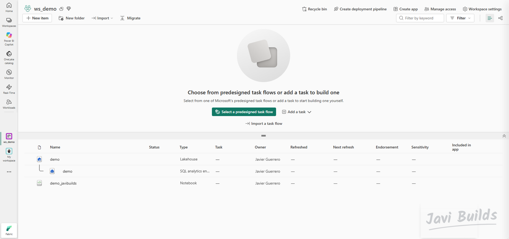
An empty workspace opens on its home page. The item list at the bottom fills up as you create the Lakehouse, notebooks and pipeline in the next steps.
 (open the full-size screenshot)
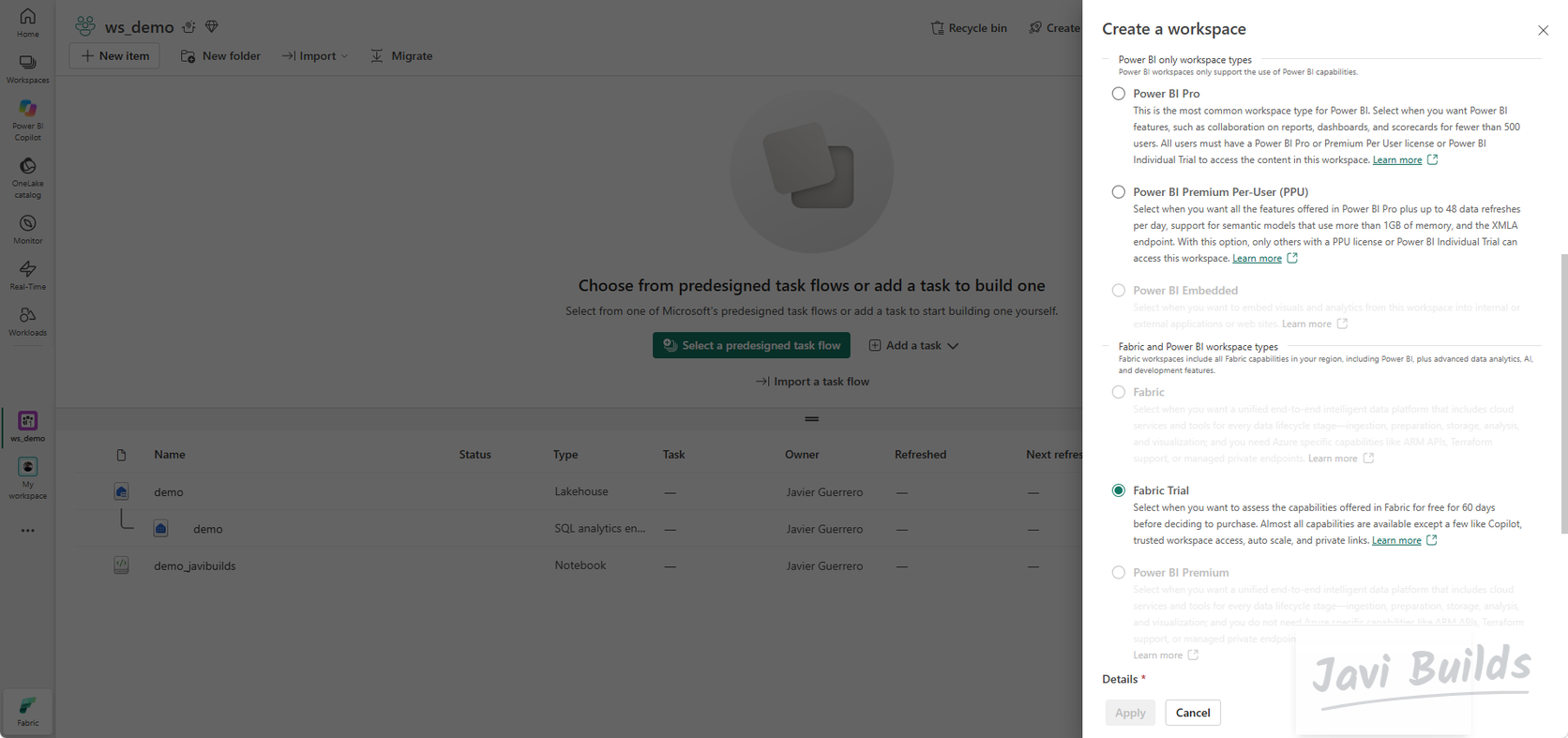
The workspace type decides which capacity runs the work. Fabric items such as Lakehouses, notebooks and pipelines need a Fabric workspace type; this build uses Fabric Trial.
 (open the full-size screenshot)
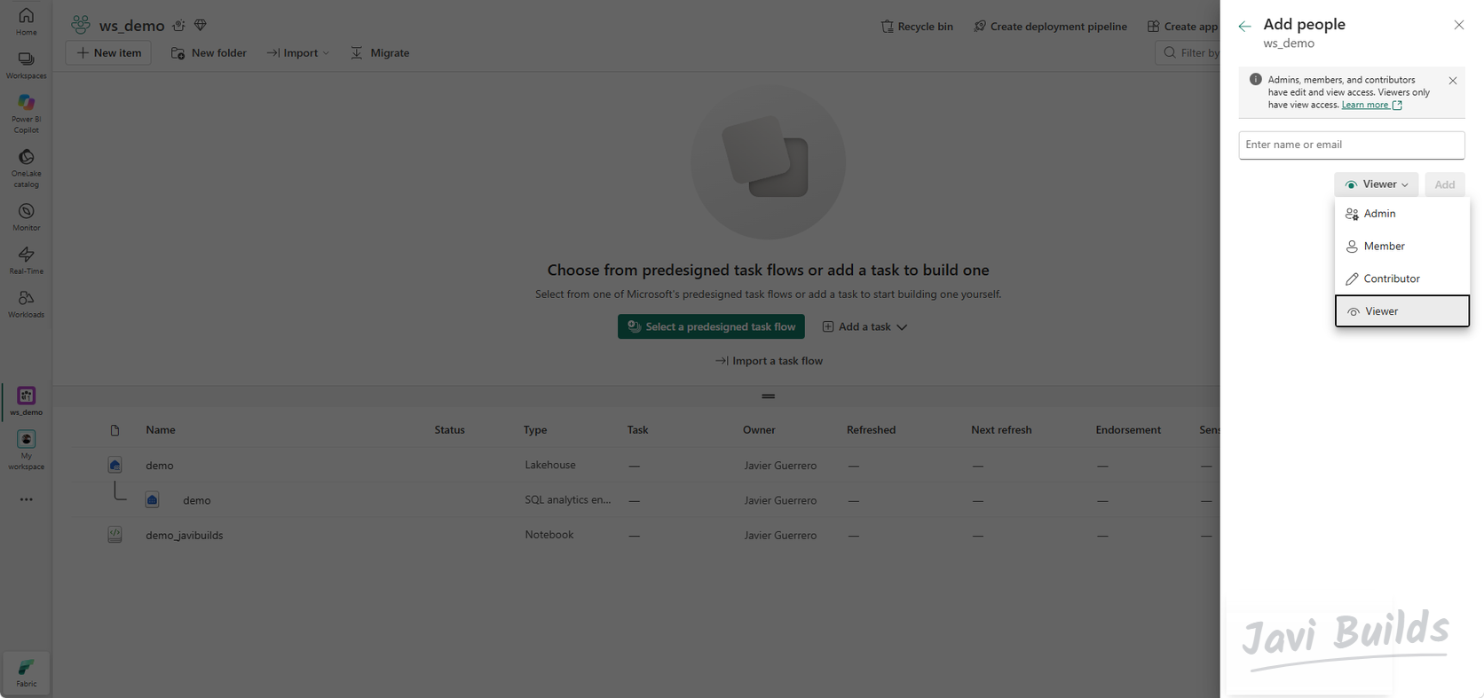
Manage access controls who can open and change the workspace. For a personal lab you can stay the only Admin; on a team, give people the narrowest role they need.
 (open the full-size screenshot)
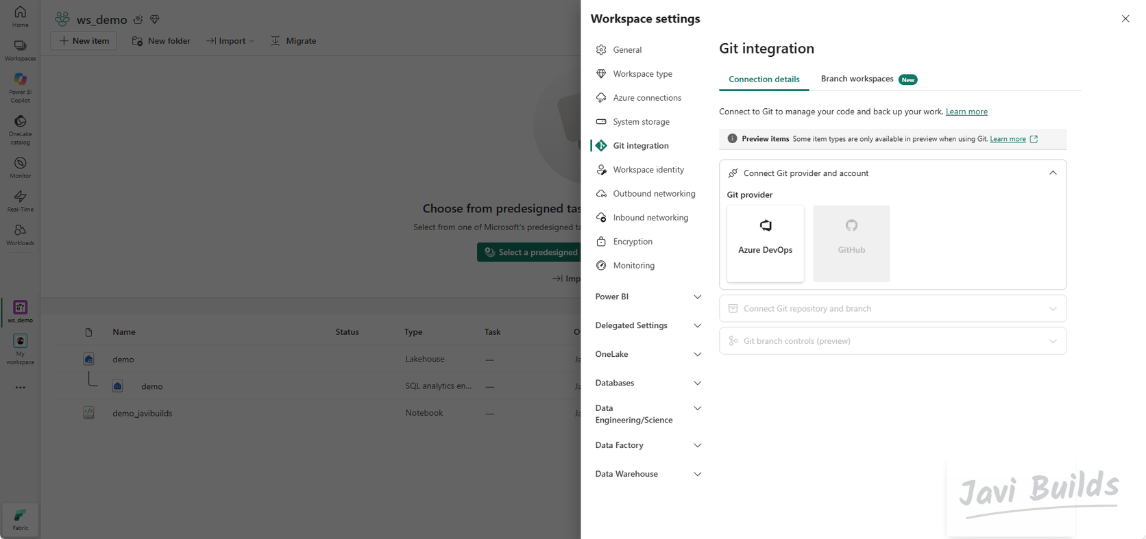
Finally, look at Workspace settings › Git integration. You do not connect Git in this lab, but knowing the workspace is Git-ready matters later: Lab 06 puts this solution under version control. For now, see connecting Fabric to Git if you want to read ahead.
 (open the full-size screenshot)
Step 2 — Create the Lakehouse
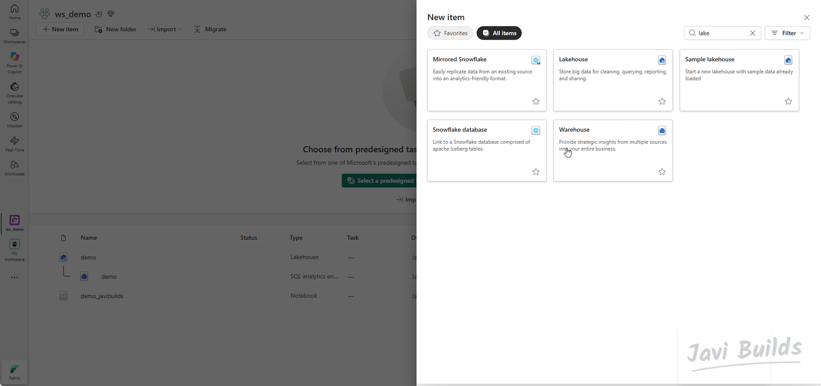
In ws_demo, select New item, search for Lakehouse and create one named demo. A Lakehouse stores data in OneLake and has two areas:
- Tables: managed Delta tables that Spark, SQL and Power BI can all read.
- Files: any files you want, in folders you choose. Raw data lands here.
 (open the full-size screenshot)
 (open the full-size screenshot)
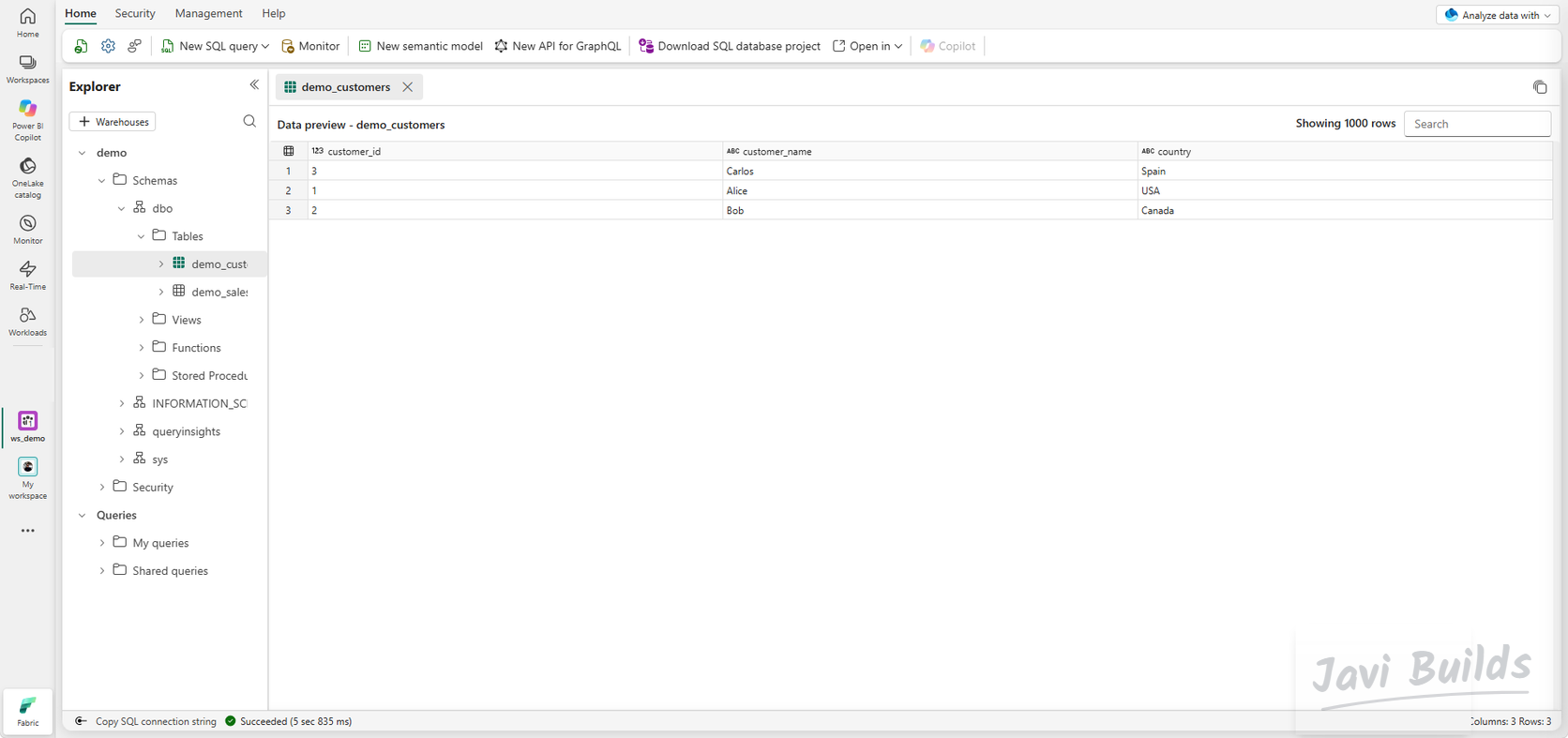
Fabric also creates a SQL analytics endpoint for every Lakehouse. It exposes the Delta tables to T-SQL in read-only mode, which is handy for checking results without opening Spark.
 (open the full-size screenshot)
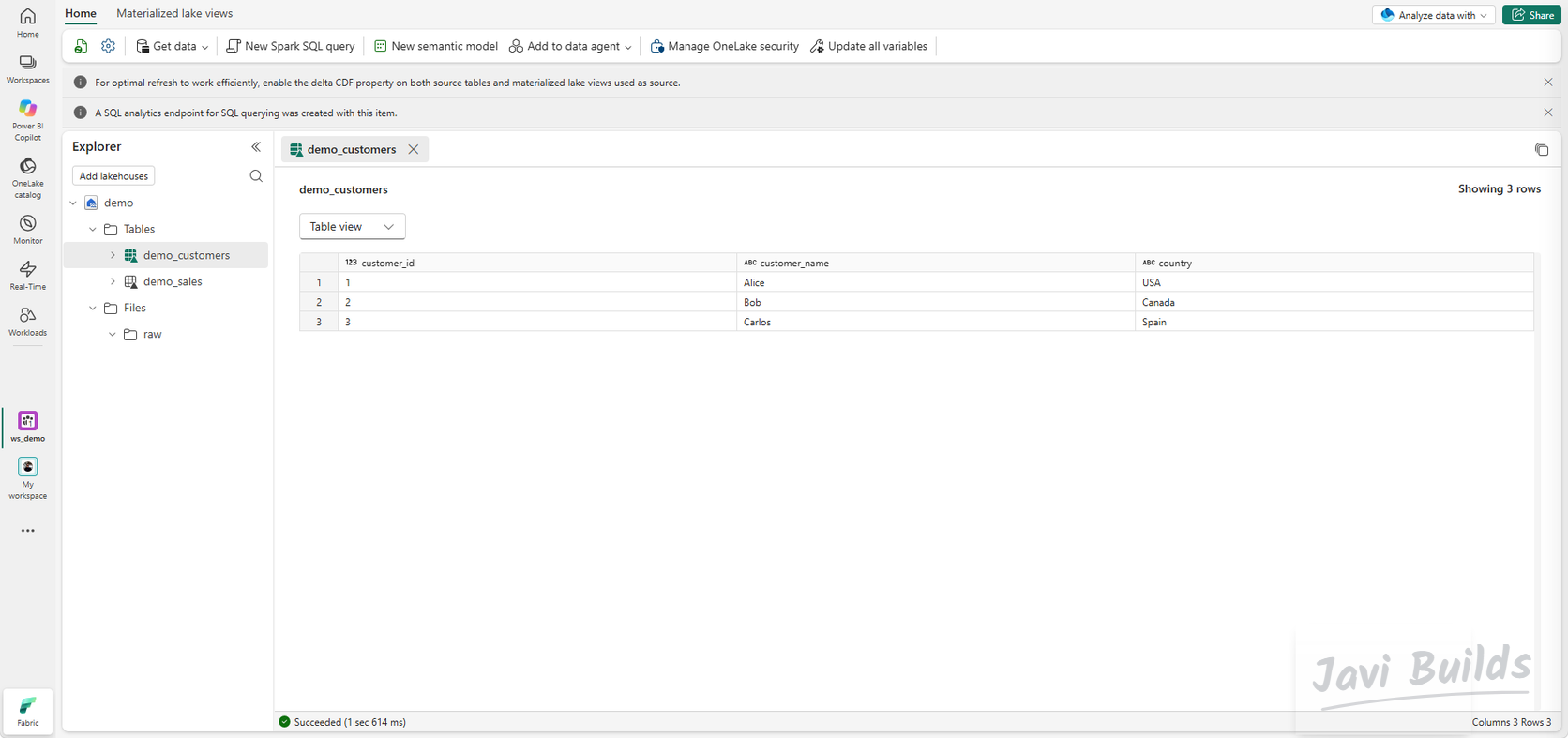
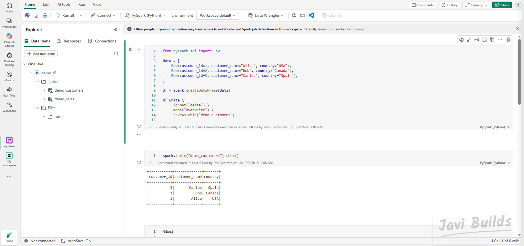
Notebooks work against an attached Lakehouse: spark.table("name") and saveAsTable("name") resolve to its Tables area. Attach demo to every notebook in this lab.
 (open the full-size screenshot)
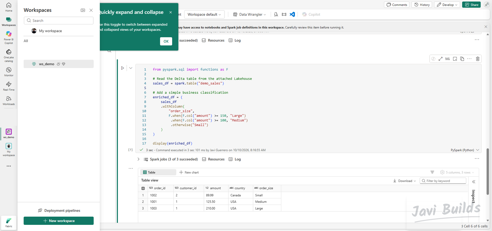
The demo_customers and demo_sales tables in these screenshots come from the Microsoft Fabric notebook tutorial. If you did not follow it, you will not have them yet; Step 7 explains where demo_sales is used. For more on Lakehouse design, see creating your first Fabric Lakehouse.
Step 3 — Load the raw data
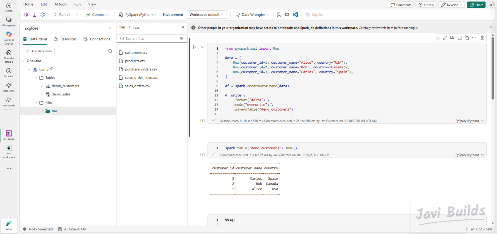
The project uses five CSV files:
customers.csvproducts.csvpurchase_orders.csvsales_orders.csvsales_order_lines.csv
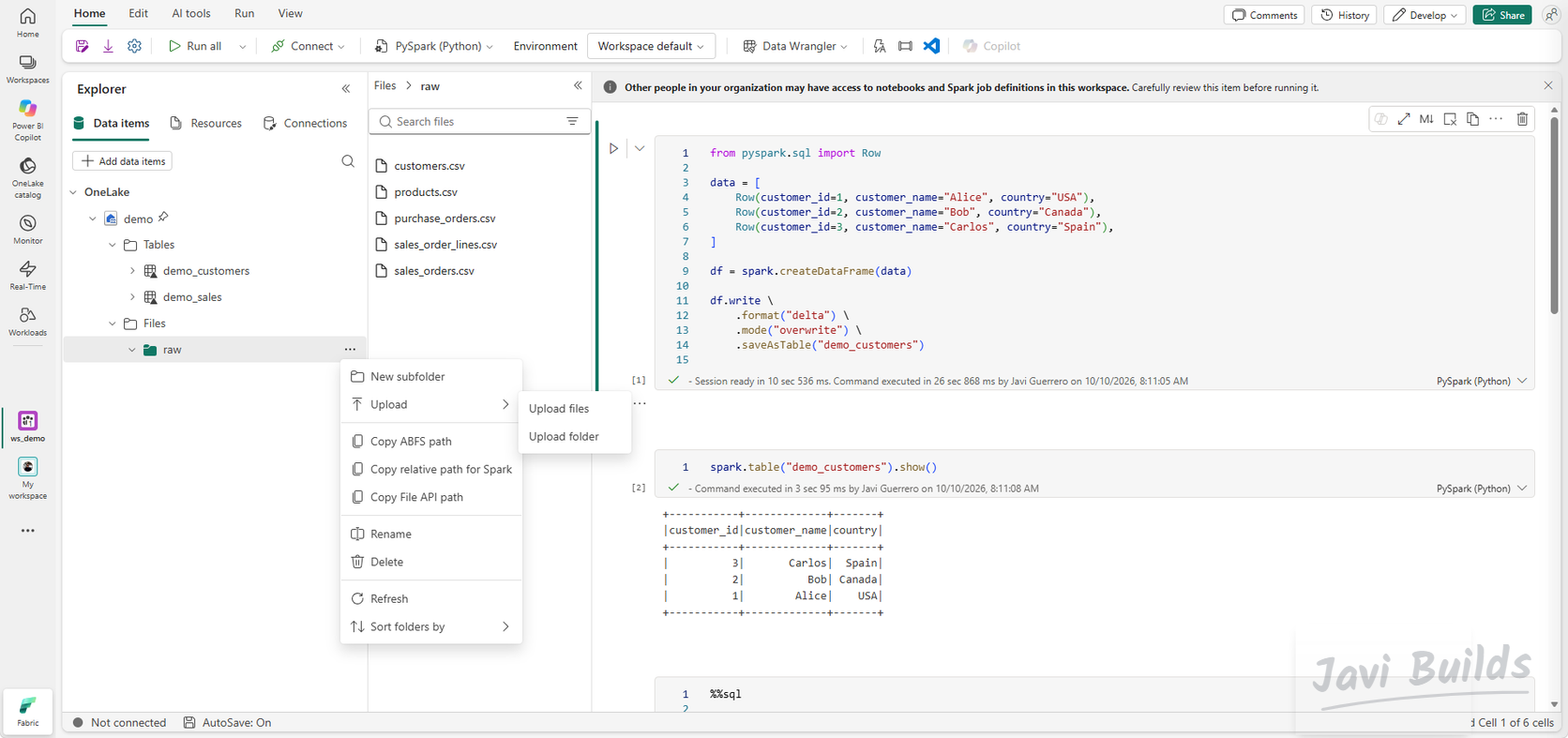
Create a folder named raw under Files, open its … menu and choose Upload › Upload files.
 (open the full-size screenshot)
Files/raw is the landing area. Files arrive here unchanged, exactly as the source produced them, and nothing downstream edits them. If a transformation goes wrong, you can always rebuild from what landed.
 (open the full-size screenshot)
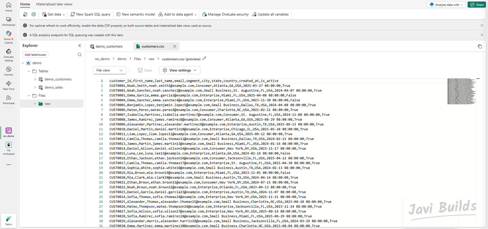
Open customers.csv to check what arrived. The header shows separate first_name and last_name columns; remember that, because it matters in Step 5.
 (open the full-size screenshot)
The sample data is synthetic: the names are generated and every email address uses the reserved example.com domain.
Step 4 — Build the Bronze layer
Create a notebook named nb_02_bronze_ingestion in ws_demo and attach the demo Lakehouse.
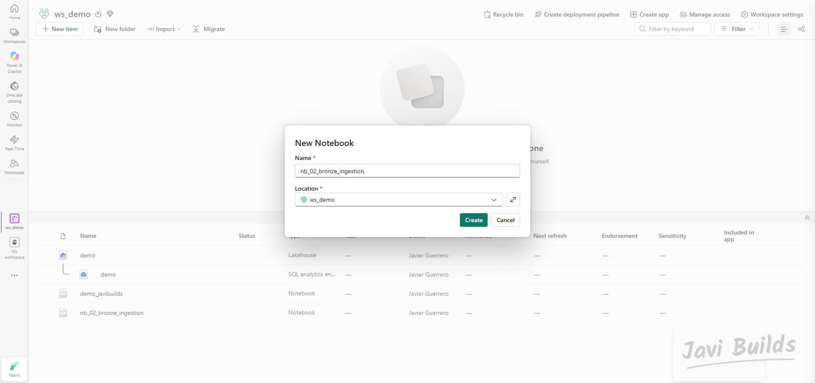 (open the full-size screenshot)
Bronze is a faithful copy of the source in Delta format, plus two columns that record where each row came from and when it arrived:
from pyspark.sql import functions as F

customers_df = (
    spark.read
    .option("header", True)
    .option("inferSchema", True)
    .csv("Files/raw/customers.csv")
    .withColumn("_source_file", F.input_file_name())
    .withColumn("_ingested_at", F.current_timestamp())
)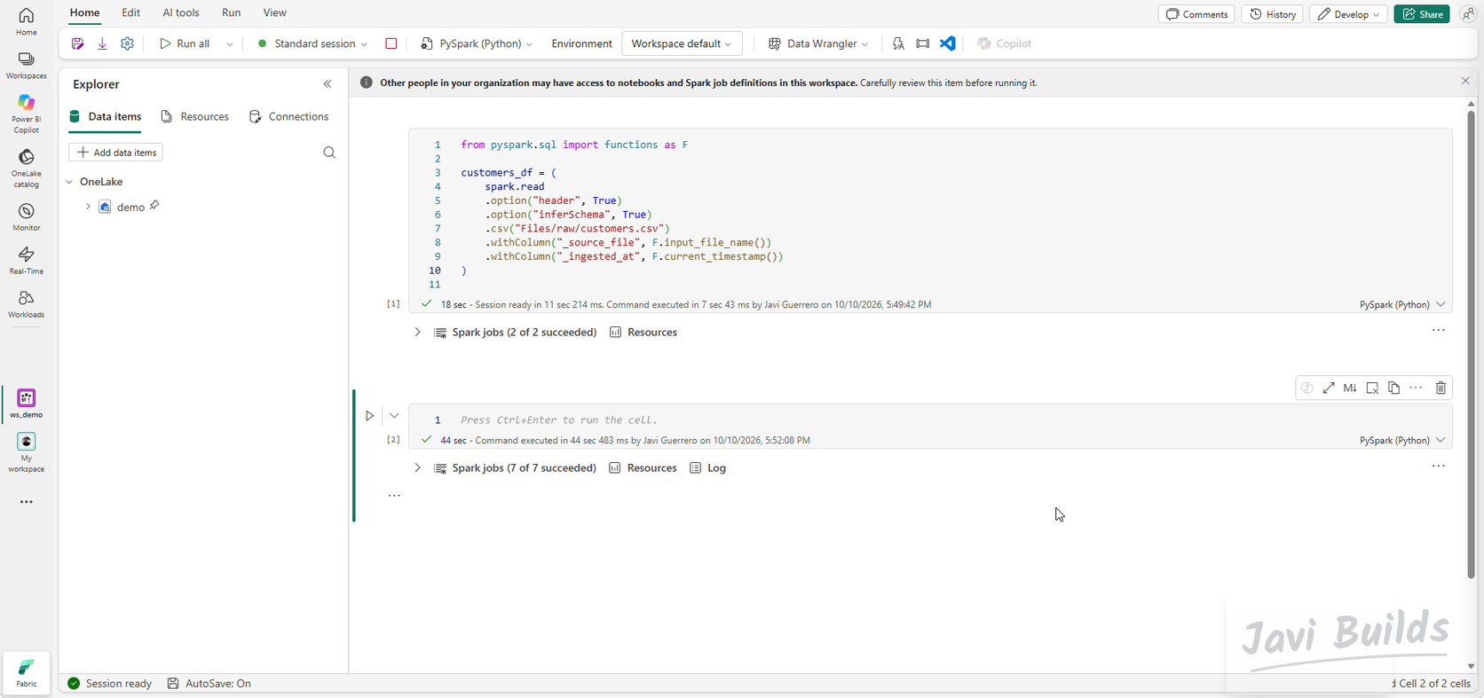 (open the full-size screenshot)
Then write the DataFrame as a Delta table:
(
    customers_df.write
    .format("delta")
    .mode("overwrite")
    .saveAsTable("bronze_customers")
)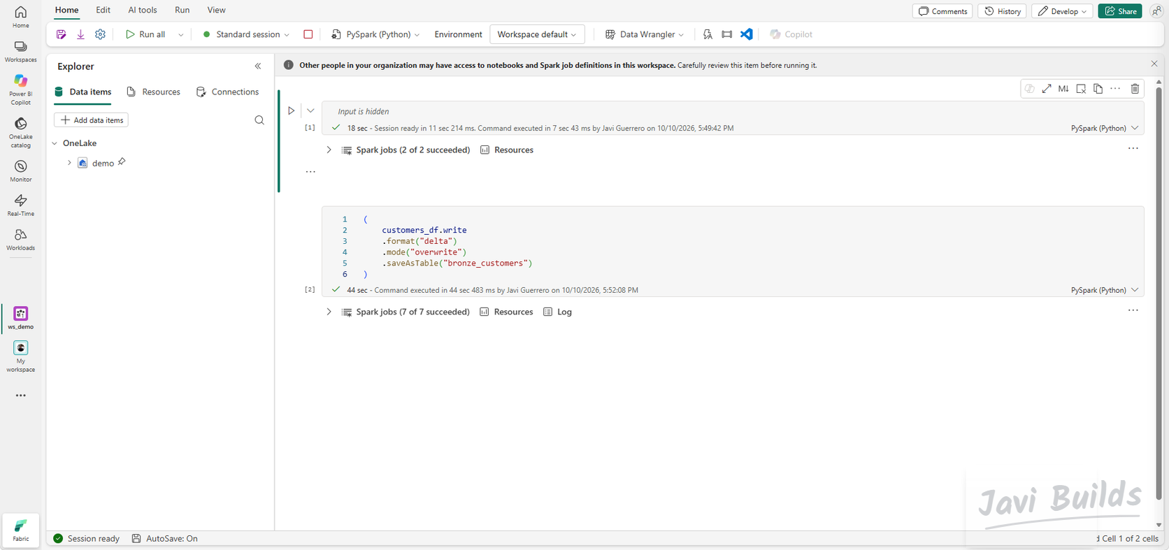 (open the full-size screenshot)
Refresh Tables: bronze_customers appears with the original columns plus _source_file and _ingested_at.
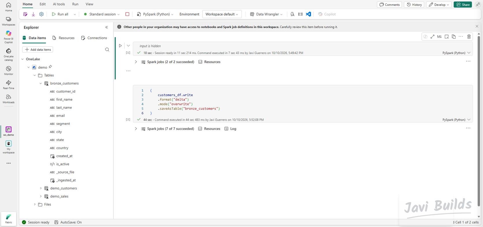 (open the full-size screenshot)
In this version of the lab, Bronze ingests customers.csv only, so that every step stays visible end to end. The other four files are landed in Files/raw but not yet loaded; repeating the same two cells for them is a good exercise. The Bronze, Silver, Gold guide explains what belongs in each layer.
Step 5 — Build the Silver layer
Create nb_03_silver_transformations and attach demo. Silver turns Bronze into clean, consistent, business-friendly data:
- Deduplication: one row per
customer_id. - Trimming: no stray spaces around names, cities or segments.
- Standardization: lowercase emails, uppercase state and country codes.
- Business-friendly columns: a single
customer_namebuilt fromfirst_nameandlast_name.
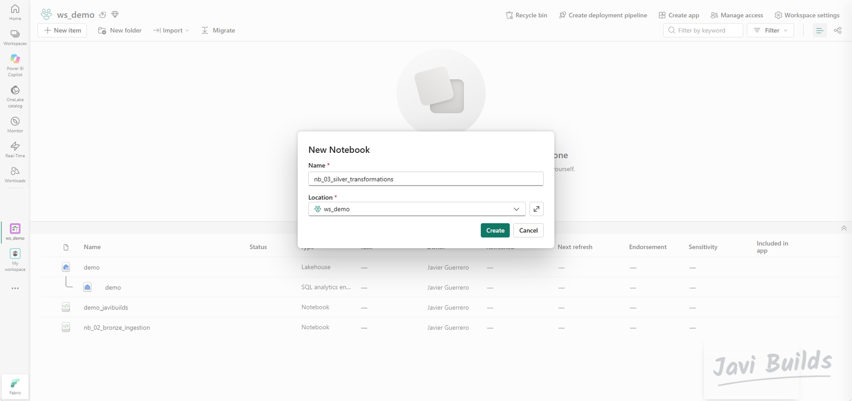 (open the full-size screenshot)
from pyspark.sql import functions as F

bronze_customers_df = spark.table("bronze_customers")

silver_customers_df = (
    bronze_customers_df
    .dropDuplicates(["customer_id"])

    # Clean first and last name
    .withColumn("first_name", F.trim(F.col("first_name")))
    .withColumn("last_name", F.trim(F.col("last_name")))

    # Create a business-friendly full name
    .withColumn(
        "customer_name",
        F.concat_ws(
            " ",
            F.col("first_name"),
            F.col("last_name")
        )
    )

    # Standardize text fields
    .withColumn("email", F.lower(F.trim(F.col("email"))))
    .withColumn("city", F.trim(F.col("city")))
    .withColumn("state", F.upper(F.trim(F.col("state"))))
    .withColumn("country", F.upper(F.trim(F.col("country"))))
    .withColumn("segment", F.trim(F.col("segment")))
)

display(silver_customers_df)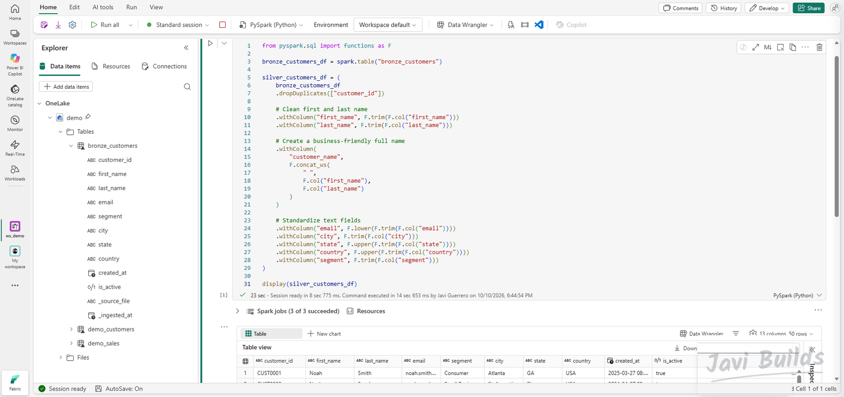 (open the full-size screenshot)
display() shows 50 rows and 13 columns: the ten source columns, the two ingestion columns and the new customer_name. Write the result to Delta:
(
    silver_customers_df.write
    .format("delta")
    .mode("overwrite")
    .saveAsTable("silver_customers")
)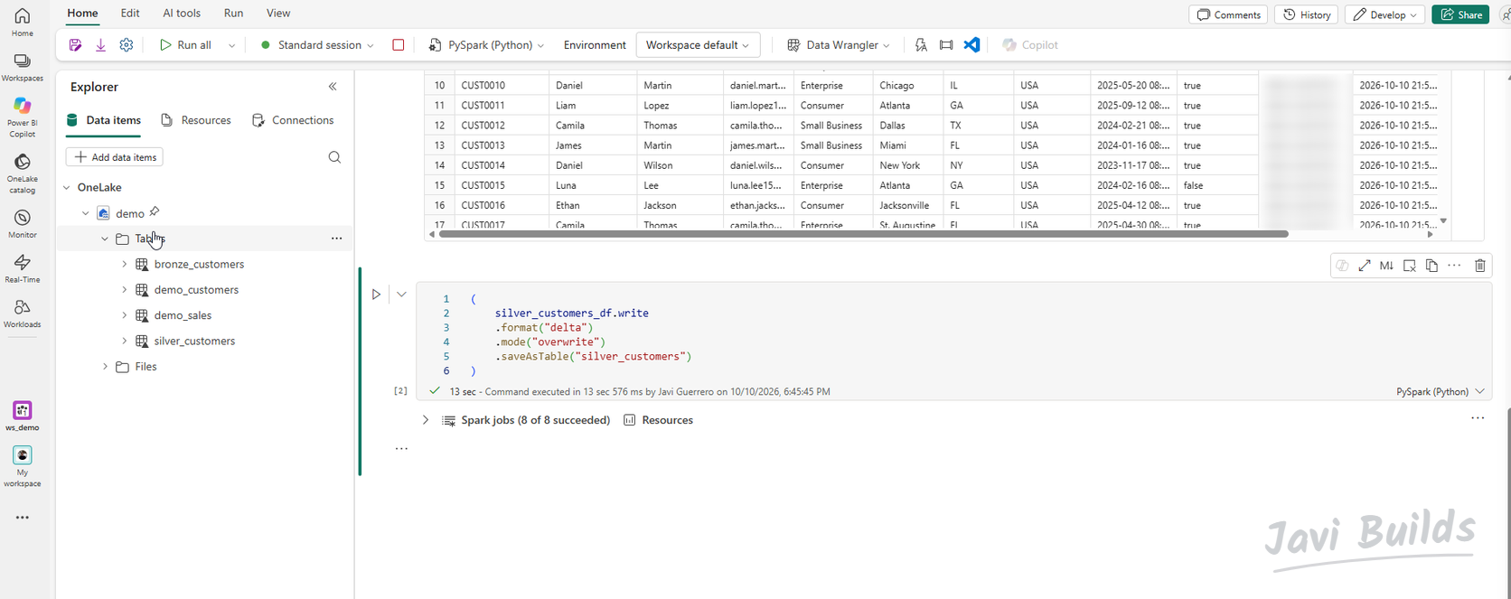 (open the full-size screenshot)
Step 6 — Data quality and troubleshooting
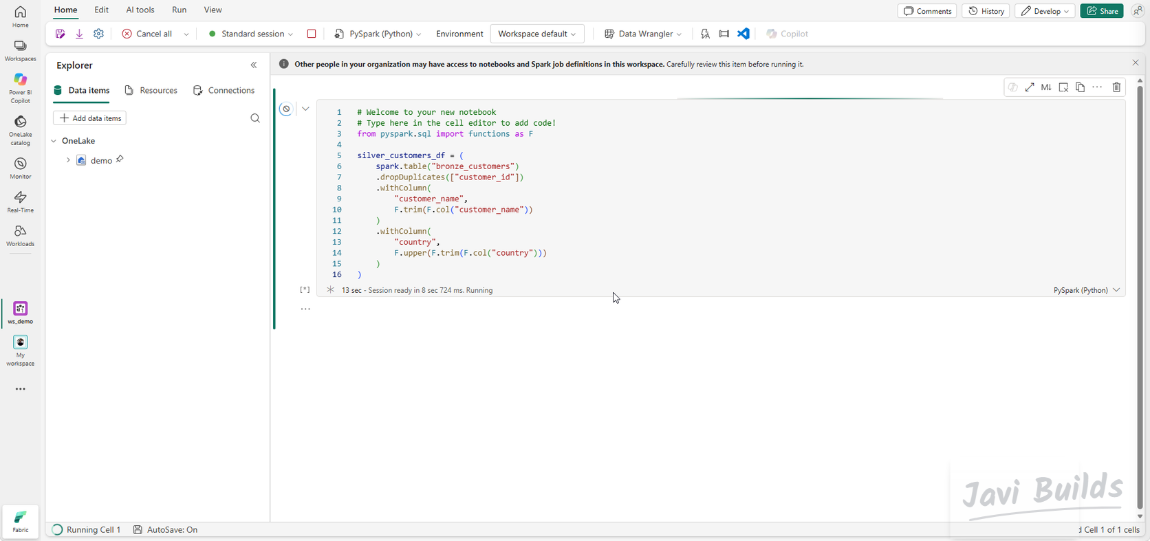
The first Silver attempt trimmed a column that was never in the source:
silver_customers_df = (
    spark.table("bronze_customers")
    .dropDuplicates(["customer_id"])
    .withColumn(
        "customer_name",
        F.trim(F.col("customer_name"))
    )
    .withColumn(
        "country",
        F.upper(F.trim(F.col("country")))
    )
) (open the full-size screenshot)
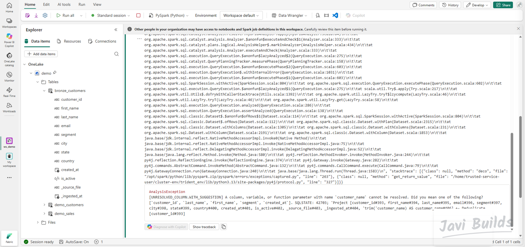
Spark rejected it before processing a single row:
 (open the full-size screenshot)
The error is [UNRESOLVED_COLUMN.WITH_SUGGESTION]: a column named customer_name cannot be resolved, and Spark suggests customer_id, last_name, first_name, segment and created_at. The fix follows a short, repeatable sequence:
- Inspect the schema. Run
spark.table("bronze_customers").printSchema(), or expand the table in the Explorer. - Identify the missing column. Bronze has
first_nameandlast_name, notcustomer_name. The raw file never had it either (Step 3). - Correct the transformation. Build
customer_namewithconcat_wsfrom the two columns that do exist, instead of reading it. - Rerun the cell.
- Verify the Silver table. Check the displayed rows, then confirm
silver_customersappears under Tables with the expected columns.
The lesson is broader than one column: Silver code should be written against the schema Bronze actually has, which is why Step 3 previews the raw file before any code depends on it.
This lab stops at fixing the transformation. Validation rules, quarantine tables for bad rows and recoverable failures are the subject of Lab 03.
Step 7 — Build the Gold layer
Create nb_04_gold_model and attach demo. Gold holds tables shaped for reporting. This lab keeps the Gold model intentionally compact, with three objects:
| Table | Role |
|---|---|
dim_customer |
Customer dimension, from the cleaned Silver customers |
fact_sales |
One row per order, with the amount and an order-size band |
gold_sales_by_country |
Pre-aggregated sales per country, ready to report |
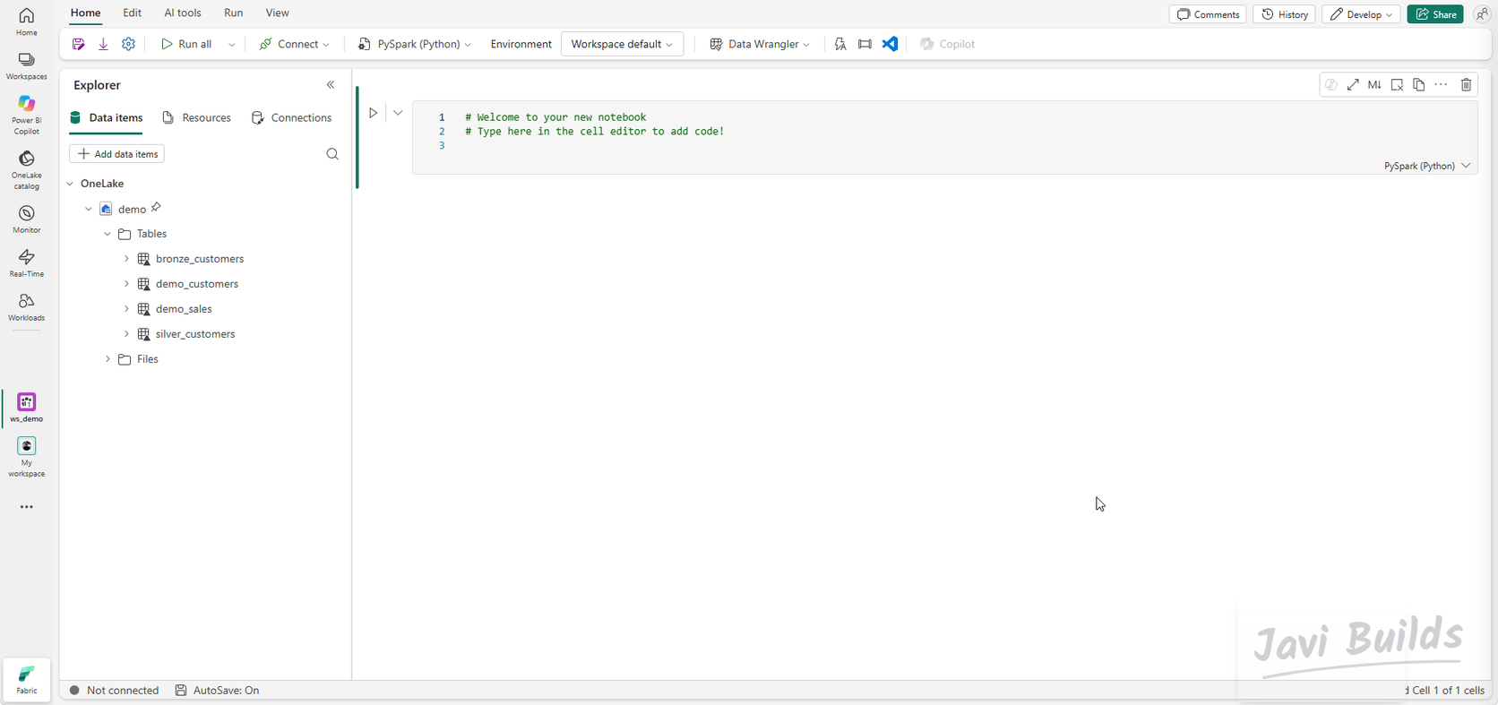 (open the full-size screenshot)
dim_customer is built from silver_customers. It keeps the descriptive customer columns, including the customer_name derived in Silver, leaves out the ingestion metadata, and guarantees one row per customer_id:
silver_customers_df = spark.table("silver_customers")

dim_customer_df = (
    silver_customers_df
    .select(
        "customer_id",
        "customer_name",
        "email",
        "segment",
        "city",
        "state",
        "country",
        "created_at",
        "is_active"
    )
    .dropDuplicates(["customer_id"])
)

(
    dim_customer_df.write
    .format("delta")
    .mode("overwrite")
    .saveAsTable("dim_customer")
)

display(dim_customer_df)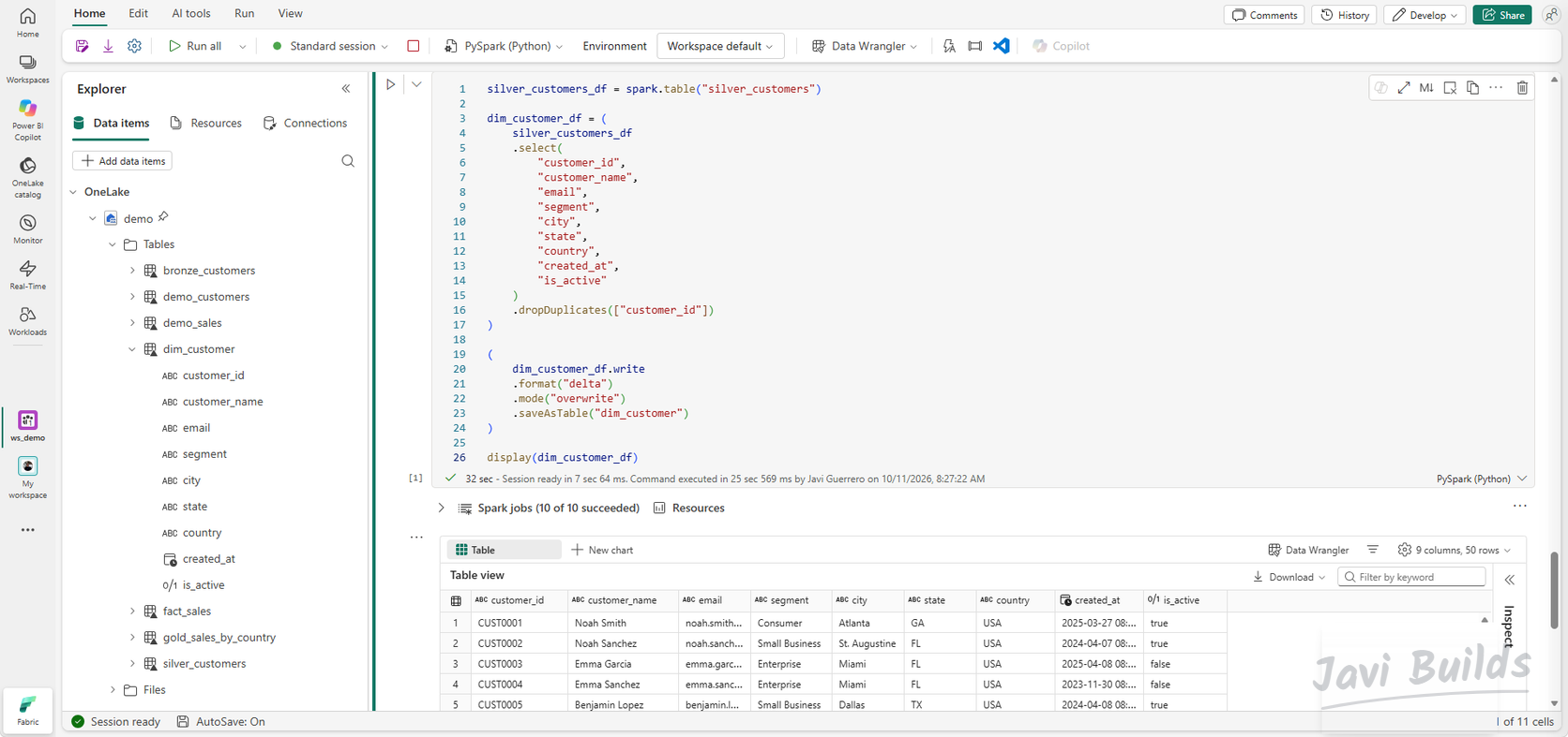 (open the full-size screenshot)
fact_sales is built from the small demo_sales table created in the notebook tutorial. It renames amount to sales_amount and adds an order-size band:
from pyspark.sql import functions as F

sales_df = spark.table("demo_sales")

fact_sales_df = (
    sales_df
    .select(
        "order_id",
        "customer_id",
        "amount",
        "country"
    )
    .withColumnRenamed(
        "amount",
        "sales_amount"
    )
    .withColumn(
        "order_size",
        F.when(F.col("sales_amount") >= 150, "Large")
         .when(F.col("sales_amount") >= 100, "Medium")
         .otherwise("Small")
    )
)

display(fact_sales_df)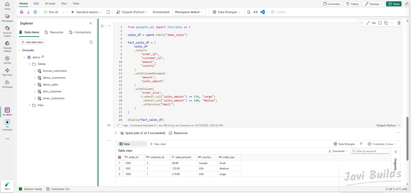 (open the full-size screenshot)
The summary table aggregates fact_sales by country:
gold_sales_by_country_df = (
    fact_sales_df
    .groupBy("country")
    .agg(
        F.countDistinct("order_id").alias("order_count"),
        F.round(F.sum("sales_amount"), 2).alias("total_sales"),
        F.round(F.avg("sales_amount"), 2).alias("avg_order_amount")
    )
    .orderBy(F.desc("total_sales"))
)

display(gold_sales_by_country_df)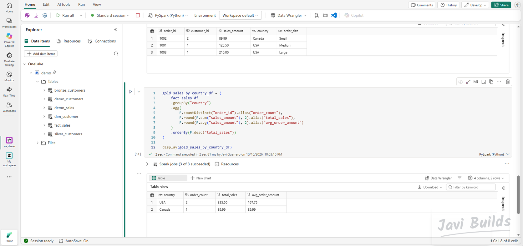 (open the full-size screenshot)
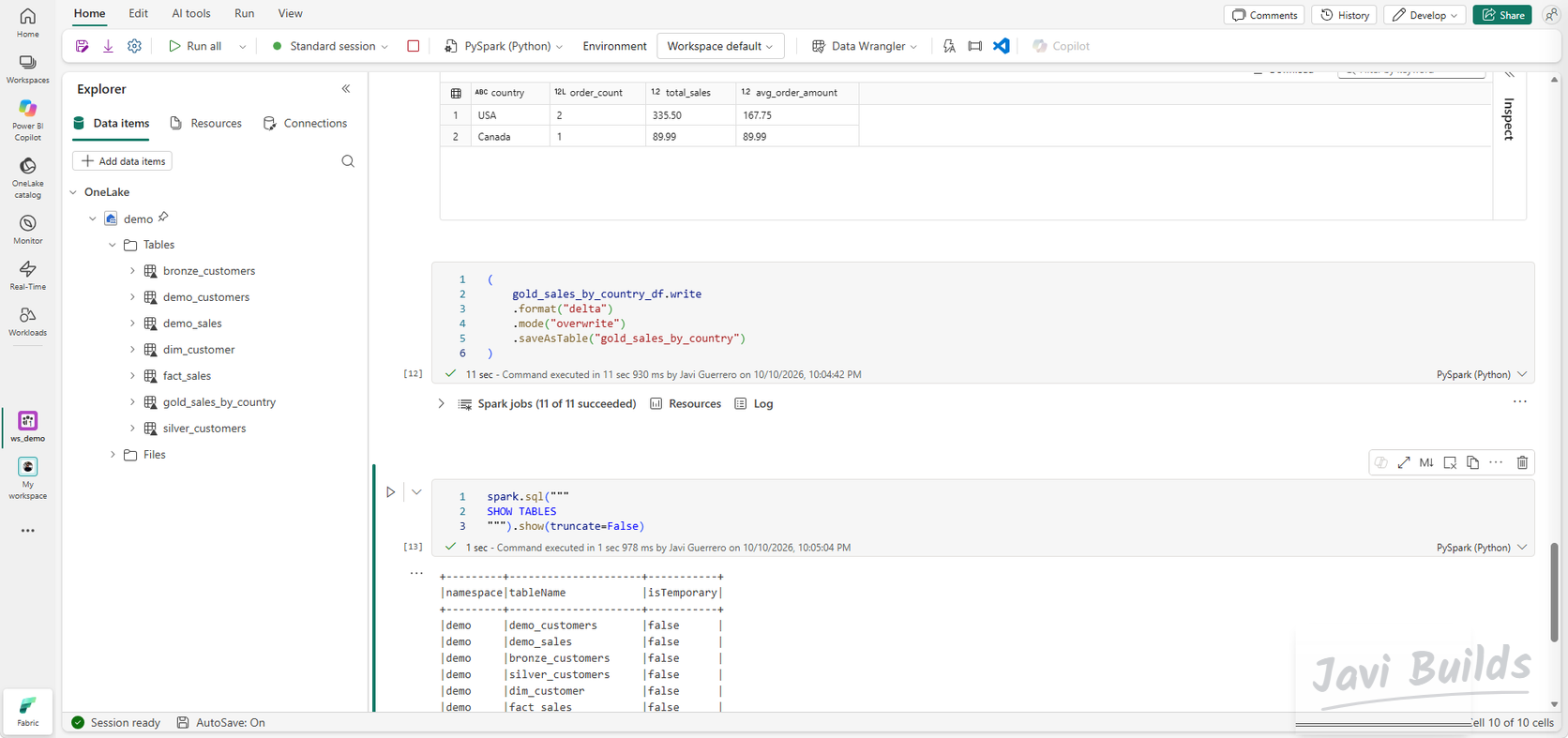
Write it with saveAsTable("gold_sales_by_country"), the same way as the earlier layers, then list the tables to confirm everything exists:
 (open the full-size screenshot)
Keep two honest limits of this Gold model in mind:
- It is a starting point, not a full production star schema. There is no product or date dimension.
fact_salescomes from the three sample orders indemo_sales, whosecustomer_idvalues (1,2) do not match theCUST…keys indim_customer. The two tables are not joinable yet. Buildingfact_salesfromsales_orders.csvandsales_order_lines.csv, with matching keys, is the natural next step, and a complete star schema is the starting point of Lab 05.
Step 8 — Orchestrate with a Fabric Pipeline
Running three notebooks by hand works once. A pipeline runs them in the right order every time and stops if a layer fails. (Why a pipeline orchestrates and the notebooks transform is explained in Pipelines vs Notebooks vs Dataflow Gen2 vs Copy Job.) Create a pipeline named pl_sales_analytics in ws_demo.
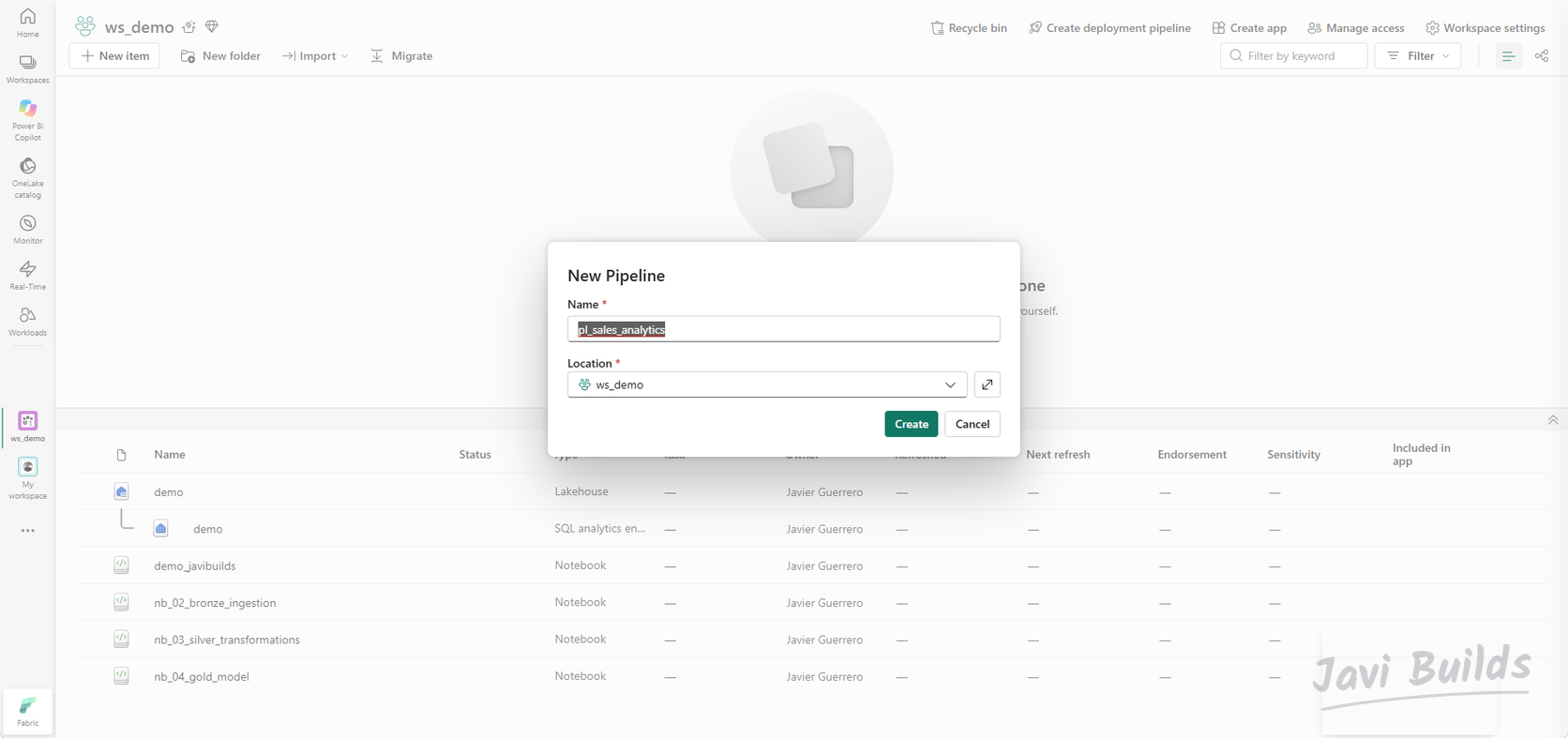 (open the full-size screenshot)
Add three Notebook activities and point each one, in its Settings tab, at its notebook:
| Activity | Notebook |
|---|---|
| Bronze Ingestion | nb_02_bronze_ingestion |
| Silver Transformations | nb_03_silver_transformations |
| Gold Model | nb_04_gold_model |
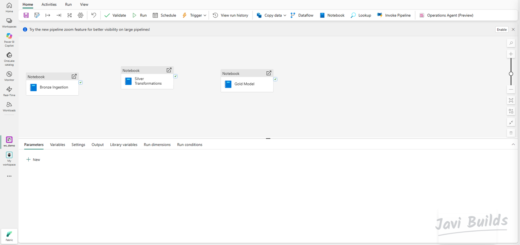 (open the full-size screenshot)
Now connect them with On success dependencies: drag from the green check of Bronze Ingestion to Silver Transformations, then from Silver Transformations to Gold Model. Silver only starts if Bronze succeeded, and Gold only if Silver succeeded, so a failure never produces a half-refreshed Gold layer.
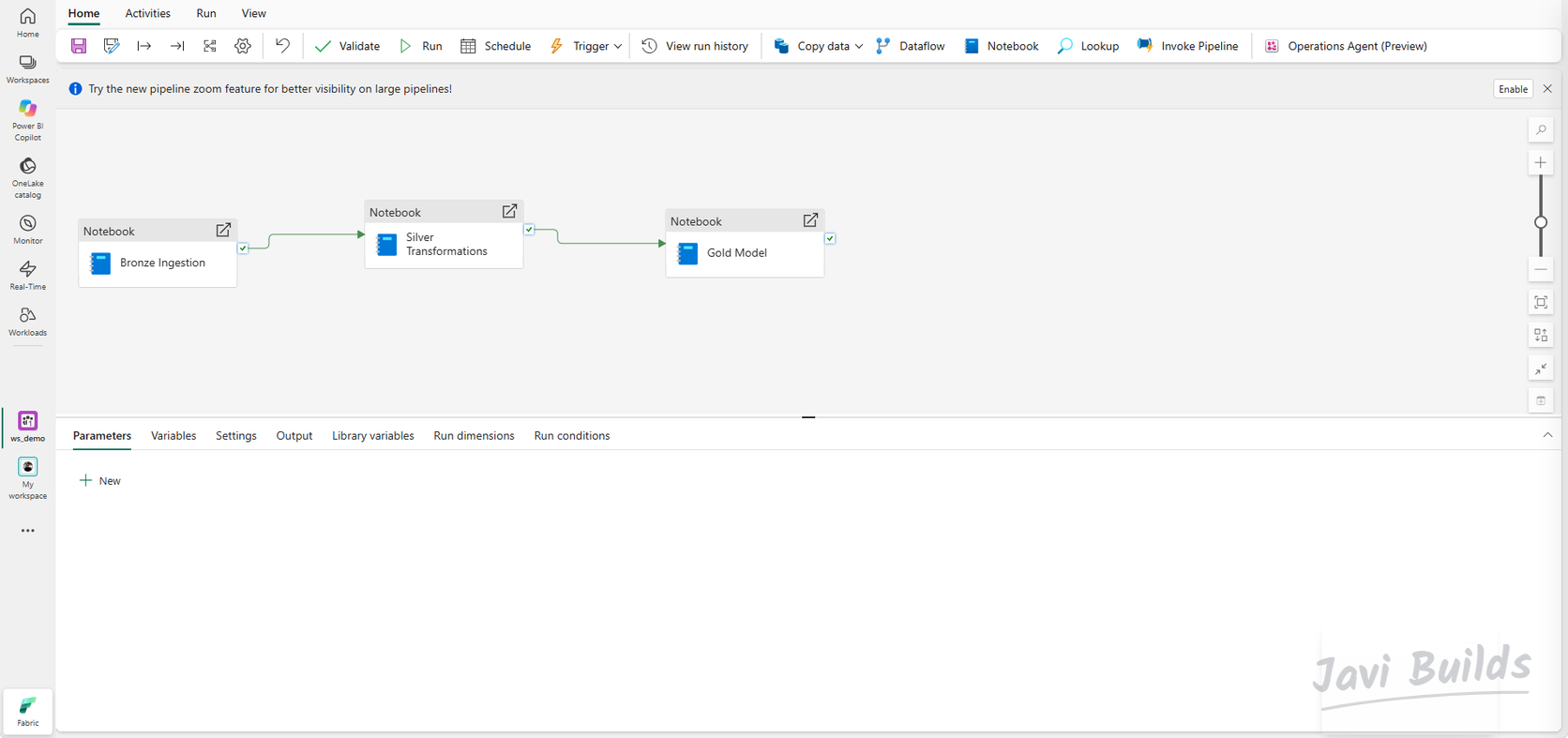 (open the full-size screenshot)
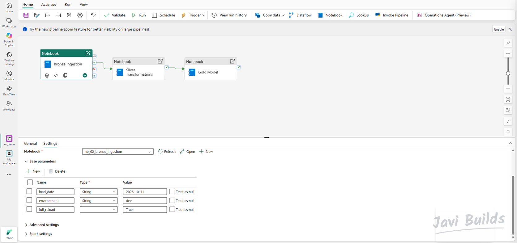
Select an activity and open its Settings tab to check which notebook it runs. The same tab has a Base parameters section, which passes values from the pipeline into the notebook. As a preview, the Bronze Ingestion activity below has three: load_date (String, 2026-10-11), environment (String, dev) and full_reload (True, with no type selected yet).
 (open the full-size screenshot)
The Bronze code from Step 4 does not read these values, so they change nothing yet: the notebook still loads customers.csv in full. Making the notebooks use them, with proper types and a parameters cell, is Lab 02.
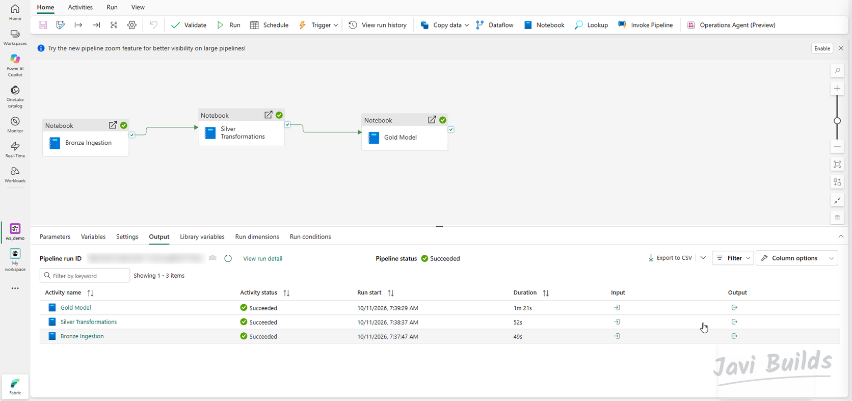
Save the pipeline and select Run. The Output tab shows each activity as it runs. In this build, all three succeeded: Bronze Ingestion in 49 seconds, Silver Transformations in 52 seconds and Gold Model in 1 minute 21 seconds.
 (open the full-size screenshot)
The pipeline’s own Parameters tab is still empty. That is intentional: hard-coded paths and full reloads keep this lab simple. Pipeline parameters, notebook parameters and incremental loads driven by load_date, environment and full_reload are the subject of Lab 02; if you want to read ahead, see Fabric notebook parameters and Incremental Loads in Microsoft Fabric, which uses this lab’s sales orders as its running example.
Result
You now have a small analytics solution that runs end to end in Microsoft Fabric:
- a Fabric workspace,
ws_demo - a Lakehouse,
demo - raw files in OneLake, under
Files/raw - a Bronze layer,
bronze_customers, with ingestion metadata - a Silver transformation,
silver_customers, cleaned and deduplicated - Gold reporting tables:
dim_customer,fact_salesandgold_sales_by_country - Fabric Pipeline orchestration with
pl_sales_analytics
- Raw CSV
- Files/rawLanding area
- Bronze
- Silver
- Gold
- Pipeline orchestration
For the reasoning behind the layers, read Medallion architecture explained. When the solution needs to record what each run did, designing an execution log for data pipelines is the background for Lab 04.
Continue learning
The next labs build on this solution. They are listed so you can see where the project is going; none of them is published yet.
Parameterized Pipelines and Incremental Processing
Pass values from the pipeline into the notebooks and load only what changed instead of reprocessing everything.
Not published yet
Data Quality, Quarantine, and Error Handling
Validate rows before they reach Silver, quarantine the ones that fail, and make failures recoverable.
Not published yet
Monitoring and Execution Logging
Record every run in a Delta execution log so you can tell what ran, what failed and how many rows moved.
Not published yet
Semantic Models and Power BI
Turn the Gold layer into a semantic model with relationships and DAX measures, then report on it in Power BI.
Not published yet
Git, CI/CD, and Deployment
Put the workspace under Git and promote the solution from development to test to production.
Not published yet