Microsoft Fabric
Microsoft Fabric Notebook Tutorial: From Your First Notebook to Production
A practical Microsoft Fabric notebook tutorial covering Lakehouse attachment, PySpark and SQL, Delta tables, parameters, pipelines, Git, monitoring, performance, and production readiness.
On this page
A Microsoft Fabric notebook can start as a few exploratory cells and quickly become part of a production data platform.
That transition is where many teams struggle.
Creating a notebook is easy. Building one that is parameterized, observable, repeatable, source-controlled, and safe to run from a pipeline requires more deliberate engineering.
This tutorial walks through that full path.
The goal is not only to show how to execute PySpark in Fabric. It is to show how a notebook fits into a real data-engineering workflow:
- Workspace
- Lakehouse
- Notebook
- Transform
- Delta tables
- Pipeline
- Monitoring
- Git / deployment
By the end, you should understand how to move from an interactive notebook to something you can operate as part of a production data platform.
What a Microsoft Fabric notebook is
A Fabric notebook is an interactive development surface for Apache Spark workloads inside Microsoft Fabric.
You can use it to:
- explore data;
- read and write Lakehouse data;
- transform large datasets with PySpark;
- execute Spark SQL;
- work with Delta tables;
- parameterize processing;
- run notebooks from Data Factory pipelines;
- integrate notebook source with Git;
- operationalize recurring data transformations.
Fabric notebooks are especially useful when the transformation needs Spark, distributed processing, or a code-first workflow.
A notebook is not automatically the best tool for every task. Simple copy operations may belong in a pipeline activity. T-SQL transformations may fit better in a Warehouse. Small orchestration steps may not need Spark at all.
The notebook is one tool in the platform.
Prerequisites
For the exercises in this tutorial, you need:
- access to a Microsoft Fabric tenant;
- a workspace assigned to Fabric capacity or an eligible trial;
- permission to create items in that workspace;
- a Lakehouse;
- a notebook.
A practical development workspace might look like:
Workspace: data-platform-dev
Lakehouse: lh_sales
Notebook: nb_transform_sales
For production environments, use separate workspaces for development, test, and production rather than treating one workspace as every environment.
Step 1: Create your first Microsoft Fabric notebook
Inside a Fabric workspace, select New item, search for Notebook, select it, and give the notebook a meaningful name such as demo_javibuilds.
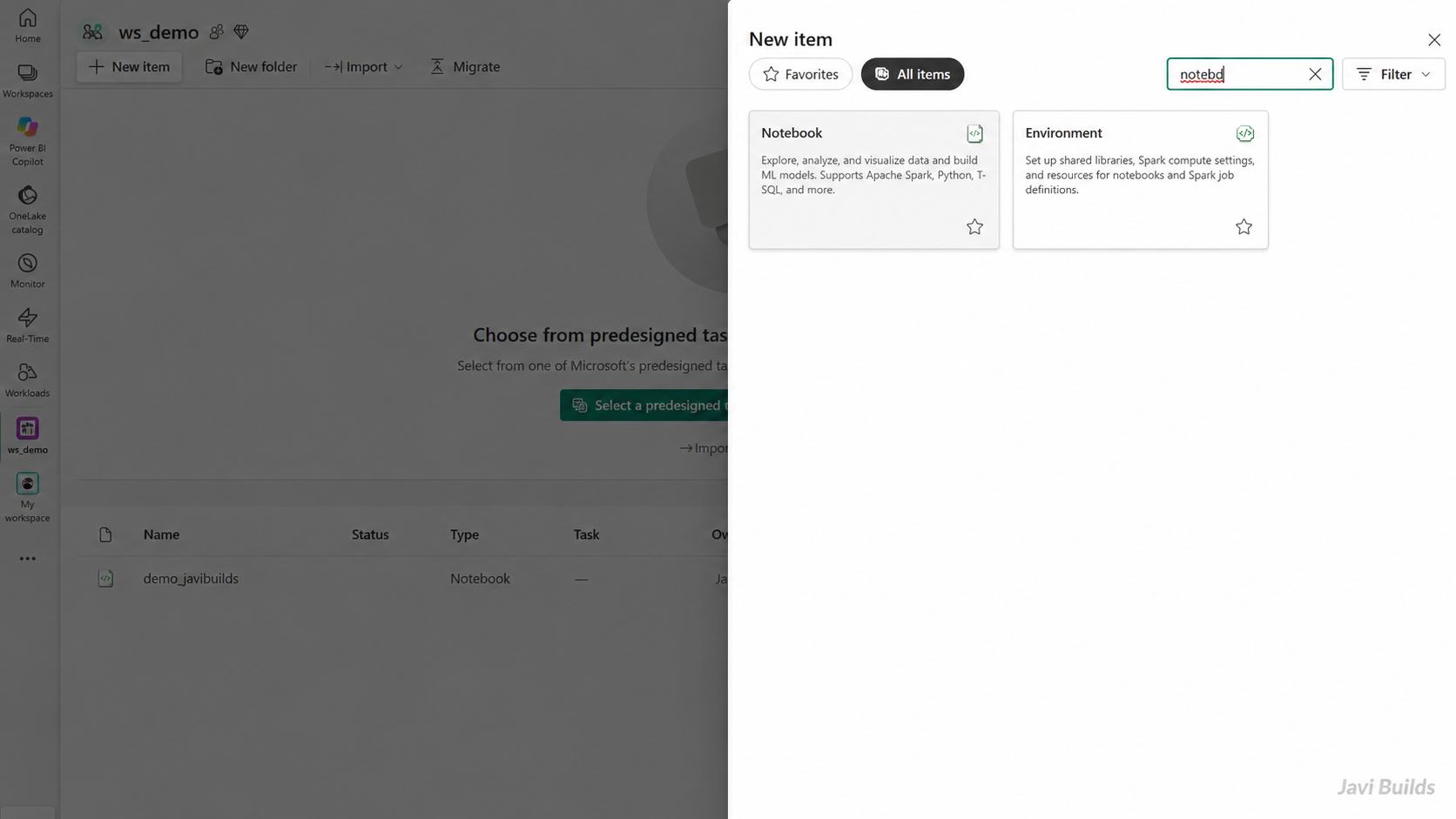
Create a Notebook from the Fabric workspace’s New item experience.
Step 2: Understand the notebook workspace
A new Fabric notebook starts with a code cell. The cell-language menu supports PySpark (Python), Spark (Scala), Spark SQL, SparkR (R), and HTML. This tutorial focuses on PySpark for DataFrame transformations and Python logic, and Spark SQL when SQL is the clearest expression of a transformation.
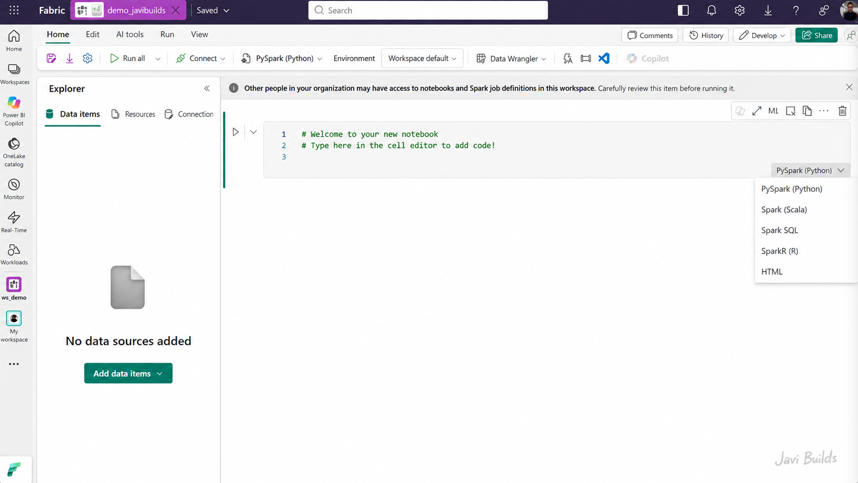
A Fabric notebook can run PySpark, Spark SQL, Scala, R, and HTML cells.
Step 3: Create or attach a Lakehouse
The Lakehouse stores the Delta tables used in this tutorial. In Data items, select Add data items and attach an existing Lakehouse or create one named demo. Once attached, Explorer exposes Tables and Files, which notebook code can read and write directly.
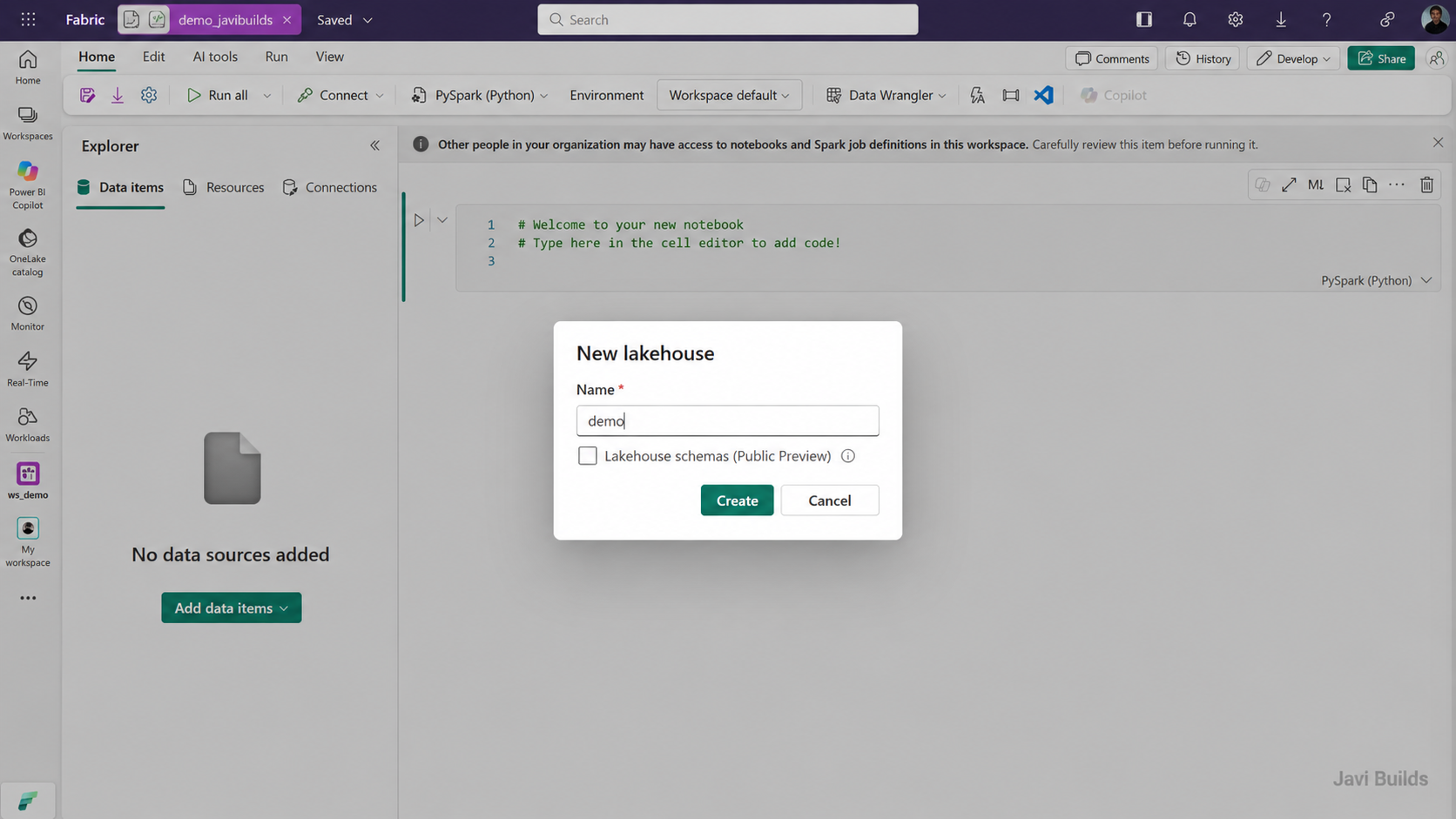
Create or attach a Lakehouse from the notebook’s Data items pane.
Step 4: How the notebook, Lakehouse, and SQL analytics endpoint fit together
Before writing more code, it helps to see how the items you just created relate to each other.
A Fabric workspace is a container for Fabric items. In this tutorial it holds the Lakehouse and the notebook you created, plus one item that Fabric created for you:
Workspace
  ├─ Lakehouse (demo)
  │   ├─ Tables
  │   ├─ Files
  │   └─ SQL analytics endpoint
  └─ Notebook (demo_javibuilds)
└─ reads/writes Delta tables in the Lakehouse- The Lakehouse is a Fabric item that stores data in OneLake, as tables and as files.
- When you create a Lakehouse, Fabric automatically creates a SQL analytics endpoint for it. The endpoint is not a second copy of the data: it exposes the Lakehouse’s Delta tables to SQL and reads the same tables in OneLake.
- The notebook is a separate item in the same workspace. It does not store the data itself; once the Lakehouse is attached, notebook code reads and writes the Lakehouse’s Delta tables and files.
- The SQL analytics endpoint lets SQL users and tools query those same Lakehouse tables with SQL, without opening a notebook. Step 11 shows it in action.
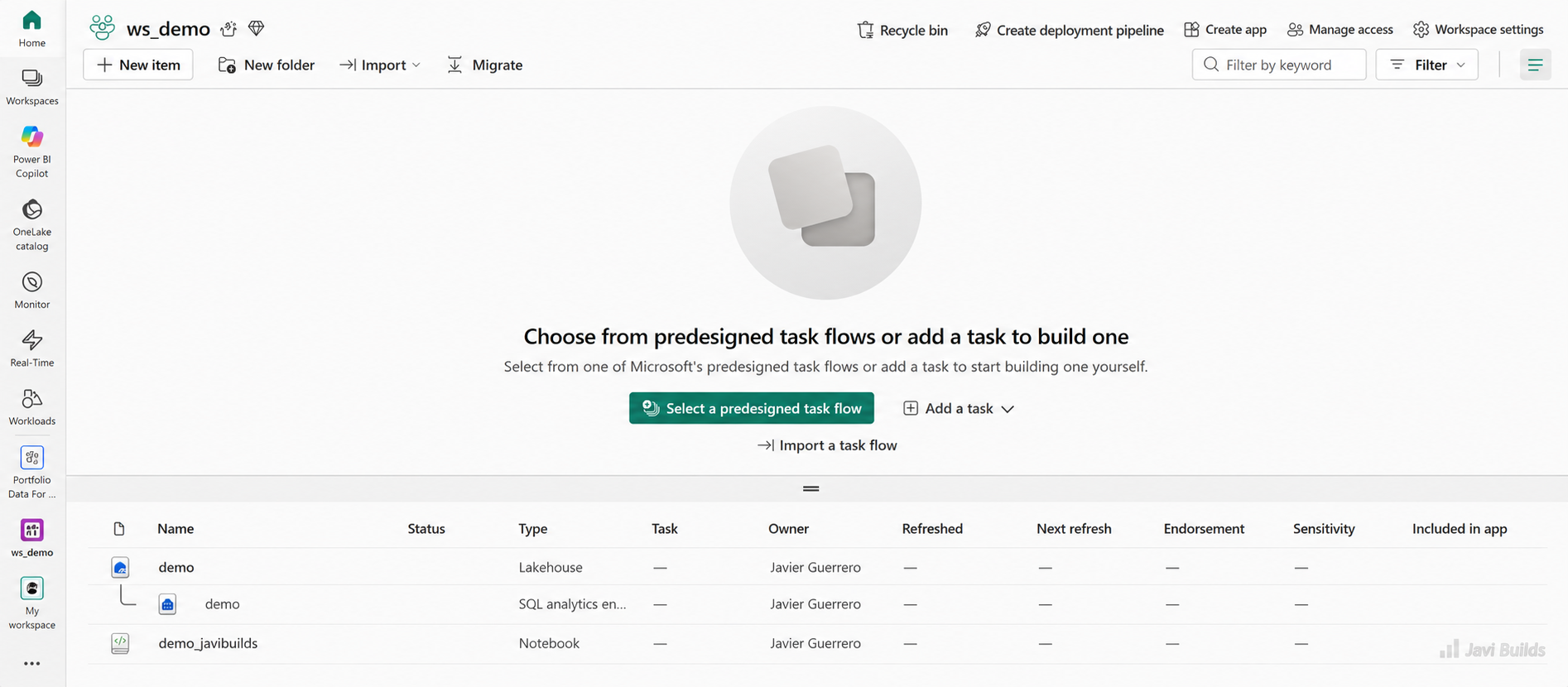
A Fabric workspace can contain the Lakehouse, its SQL analytics endpoint, and the Notebook that processes its data.
Step 5: Tables and Files inside a Fabric Lakehouse
The Lakehouse Explorer shows two areas: Tables and Files. Both live in OneLake, but they serve different purposes.
Tables
- managed Delta tables that you can query;
- visible to Spark by name, for example
spark.table("demo_customers"); - queryable through the SQL analytics endpoint;
- appropriate for structured, curated data such as
demo_customersanddemo_sales.
Files
- general-purpose file storage in OneLake;
- useful for CSV, JSON, Parquet, and other formats;
- often used for raw landing or staging data;
- a file in Files does not automatically become a managed Lakehouse table: you load it into a table, for example with
saveAsTable().
| Tables | Files | |
|---|---|---|
| Holds | Managed Delta tables | Files in any format (CSV, JSON, Parquet, …) |
| Read from Spark | spark.table("demo_customers") |
spark.read.csv("Files/raw/customers.csv") |
| SQL analytics endpoint | Queryable as tables | Not exposed as tables |
| Typical use | Structured, curated data | Raw landing and staging data |
The screenshot below shows the Lakehouse after the next steps: demo_customers and demo_sales under Tables, and a raw folder under Files.
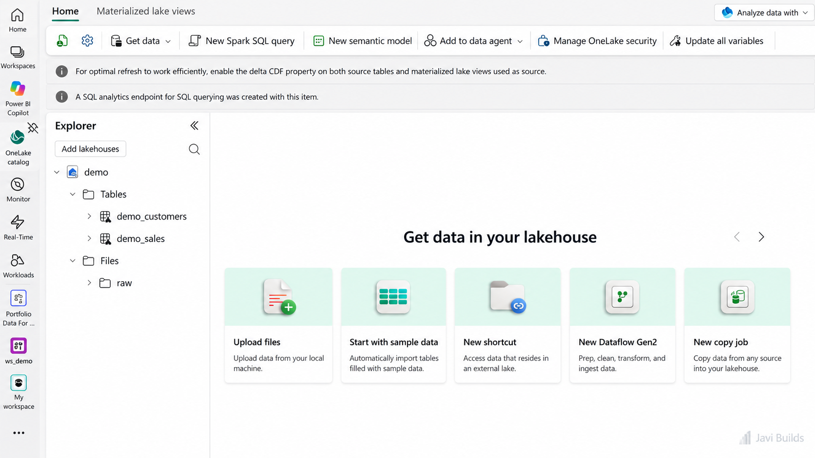
A Fabric Lakehouse separates managed tables from general file storage while keeping both in OneLake.
Step 6: Create a Delta table with PySpark
Create a small Spark DataFrame and save it as a managed Delta table in the attached Lakehouse. (How Delta tables differ from SQL Server tables covers what a Delta table is under the hood.)
from pyspark.sql import Row

data = [
    Row(customer_id=1, customer_name="Alice", country="USA"),
    Row(customer_id=2, customer_name="Bob", country="Canada"),
    Row(customer_id=3, customer_name="Carlos", country="Spain"),
]

df = spark.createDataFrame(data)

df.write \
    .format("delta") \
    .mode("overwrite") \
.saveAsTable("demo_customers")Verify the table:
spark.table("demo_customers").show()createDataFrame() creates the Spark DataFrame, format("delta") selects Delta format, and saveAsTable("demo_customers") registers the table under Tables in the attached Lakehouse.
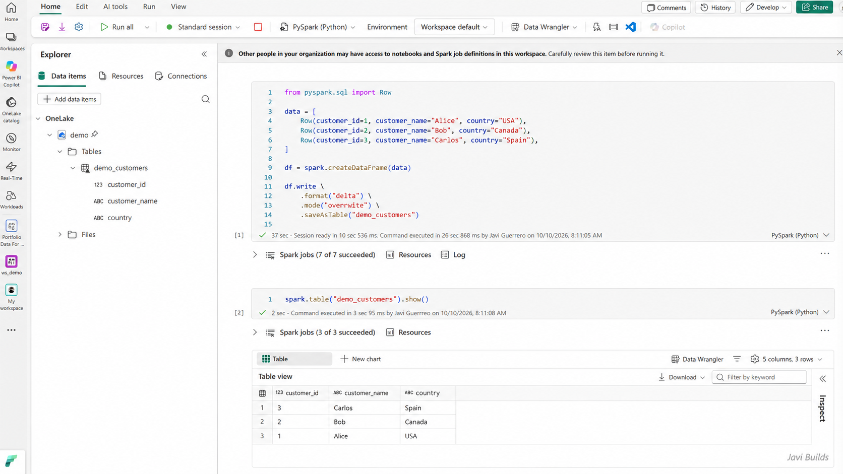
PySpark creates demo_customers as a Delta table in the attached Lakehouse.
Step 7: Create and query the table with Spark SQL
You can create the same Delta table with Spark SQL. This is Spark SQL running on the notebook Spark session—not the Fabric Warehouse SQL endpoint or SQL Server T-SQL. Step 11 shows the Lakehouse’s own SQL analytics endpoint.
CREATE OR REPLACE TABLE demo_customers
USING DELTA
AS
SELECT 1 AS customer_id, 'Alice' AS customer_name, 'USA' AS country
UNION ALL
SELECT 2, 'Bob', 'Canada'
UNION ALL
SELECT 3, 'Carlos', 'Spain';Then query it:
SELECT *
FROM demo_customers;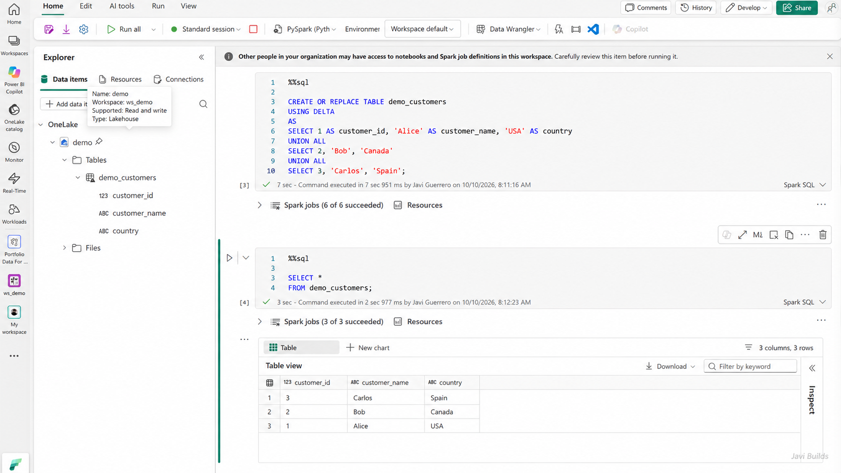
Spark SQL can create and query the same Delta table without leaving the notebook.
PySpark vs. Spark SQL: Both execute on Spark and can work with the same Delta tables. Use PySpark when transformations are easier to express with DataFrames and Python logic; use Spark SQL when SQL is clearest.
Step 8: Create sample sales data
Create a second Delta table so the tutorial has realistic data to transform:
CREATE OR REPLACE TABLE demo_sales
USING DELTA
AS
SELECT 1001 AS order_id, 1 AS customer_id, 125.50 AS amount, 'USA' AS country
UNION ALL
SELECT 1002, 2, 89.99, 'Canada'
UNION ALL
SELECT 1003, 1, 210.00, 'USA';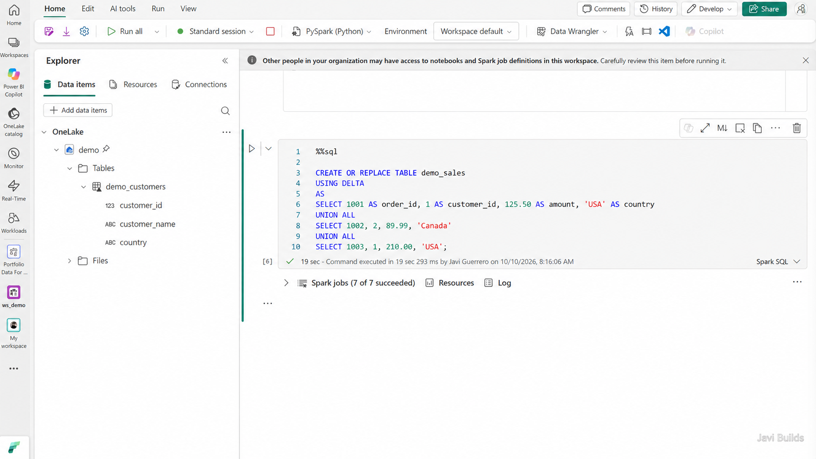
A second Delta table gives us data we can transform with PySpark.
Step 9: Transform Lakehouse data with PySpark
Read demo_sales, add a derived business classification, and inspect the result:
from pyspark.sql import functions as F

sales_df = spark.table("demo_sales")

enriched_df = (
    sales_df
    .withColumn(
        "order_size",
        F.when(F.col("amount") >= 150, "Large")
         .when(F.col("amount") >= 100, "Medium")
         .otherwise("Small")
    )
)

display(enriched_df)The code reads a Delta table from the attached Lakehouse, adds order_size, and displays the transformed DataFrame interactively.
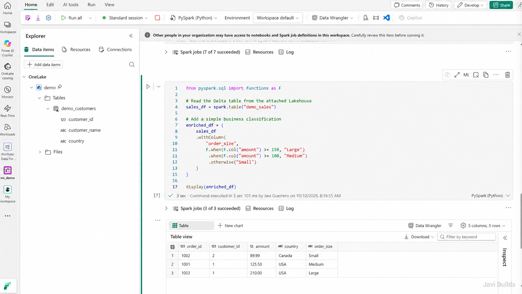
Read a Lakehouse Delta table with PySpark, add a derived column, and inspect the result interactively.
The attached Lakehouse stays visible in the notebook’s Explorer while you work, so you can see the Delta tables the code reads, such as demo_sales, next to the transformed rows:
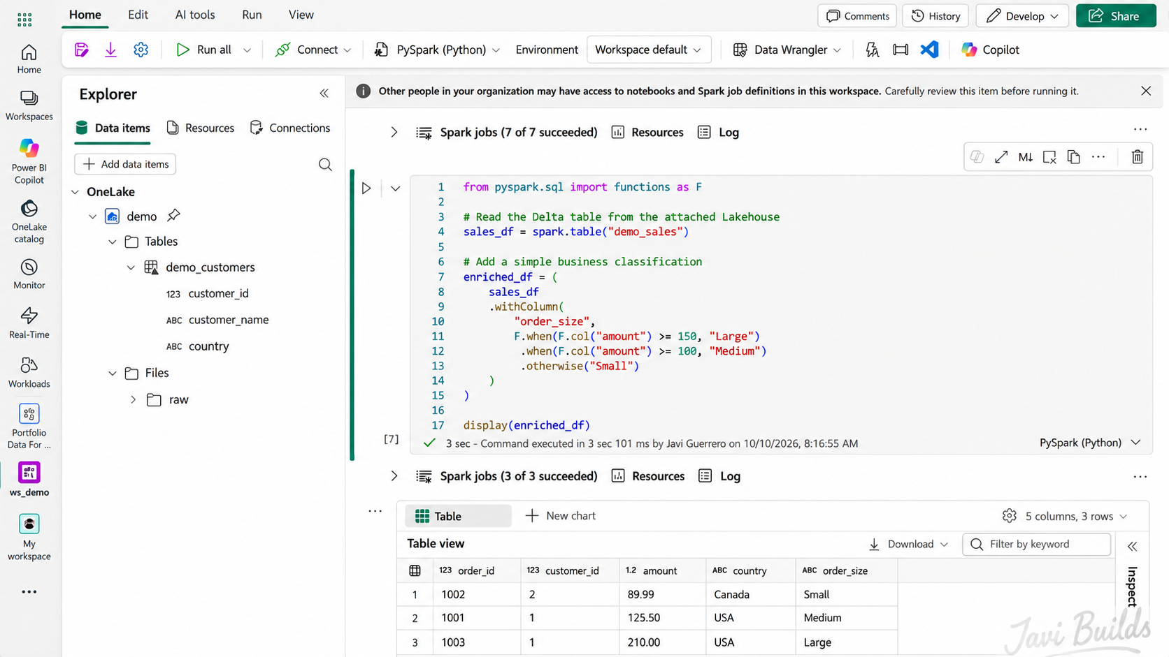
With the Lakehouse attached, PySpark can read Delta tables directly and display transformed results in the same notebook.
Aggregate the result by country:
country_summary_df = (
    enriched_df
    .groupBy("country")
    .agg(
        F.count("*").alias("order_count"),
        F.round(F.sum("amount"), 2).alias("total_sales"),
        F.round(F.avg("amount"), 2).alias("avg_order_amount")
    )
    .orderBy(F.desc("total_sales"))
)

display(country_summary_df)Persist the reusable summary in the Lakehouse:
(
    country_summary_df.write
    .format("delta")
    .mode("overwrite")
    .saveAsTable("demo_sales_by_country")
)overwrite is convenient for a tutorial, but production workloads may need append, partition replacement, MERGE, incremental processing, or idempotent updates. Always ask what happens when the notebook runs twice.
Step 10: Land raw files in Files/raw
Real pipelines rarely start from hand-typed rows. Source systems usually deliver files, and the Lakehouse Files area is a natural place to land them before they become Delta tables.
One possible organization:
Files/raw/
  customers.csv
  products.csv
  purchase_orders.csv
  sales_order_lines.csv
  sales_orders.csv
This is an example layout, not a Fabric requirement. Choose folders that match your sources and retention needs, for example by source system, by load date, or by tenant.
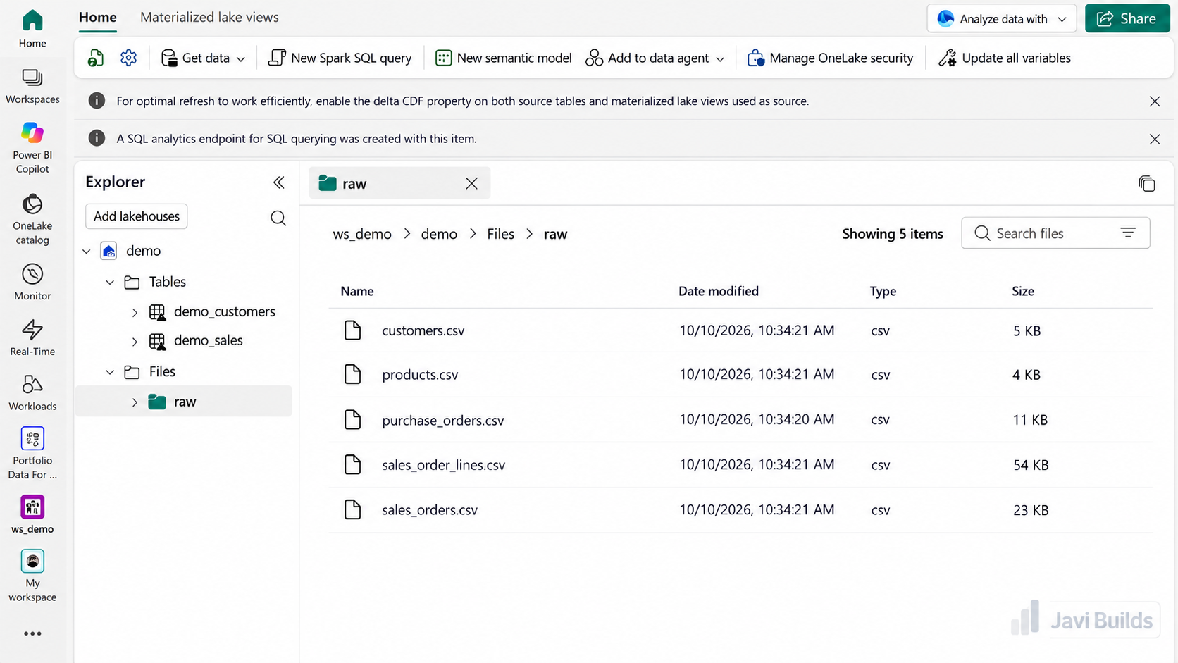
The Files area is a natural place to land raw source files before transforming them into Delta tables.
Read one of the files with PySpark:
raw_customers_df = (
    spark.read
    .option("header", True)
    .option("inferSchema", True)
    .csv("Files/raw/customers.csv")
)

display(raw_customers_df)inferSchema is convenient for exploring a file. For production ingestion, declare an explicit schema with .schema(...) so that a type change in the source is caught instead of silently inferred.
Then load it into a managed Delta table:
(
    raw_customers_df.write
    .format("delta")
    .mode("overwrite")
    .saveAsTable("demo_customers_from_file")
)After this write, demo_customers_from_file appears under Tables, and the CSV file stays in Files/raw/. The file itself did not become a table: the notebook created a new Delta table from it.
Step 11: Query Lakehouse tables through the SQL analytics endpoint
The Delta tables you created are not only for Spark. Open the Lakehouse’s SQL analytics endpoint from the workspace, or switch the Lakehouse view to SQL analytics endpoint, and query the tables with SQL:
SELECT TOP (100)
    customer_id,
    customer_name,
    country
FROM dbo.demo_customers;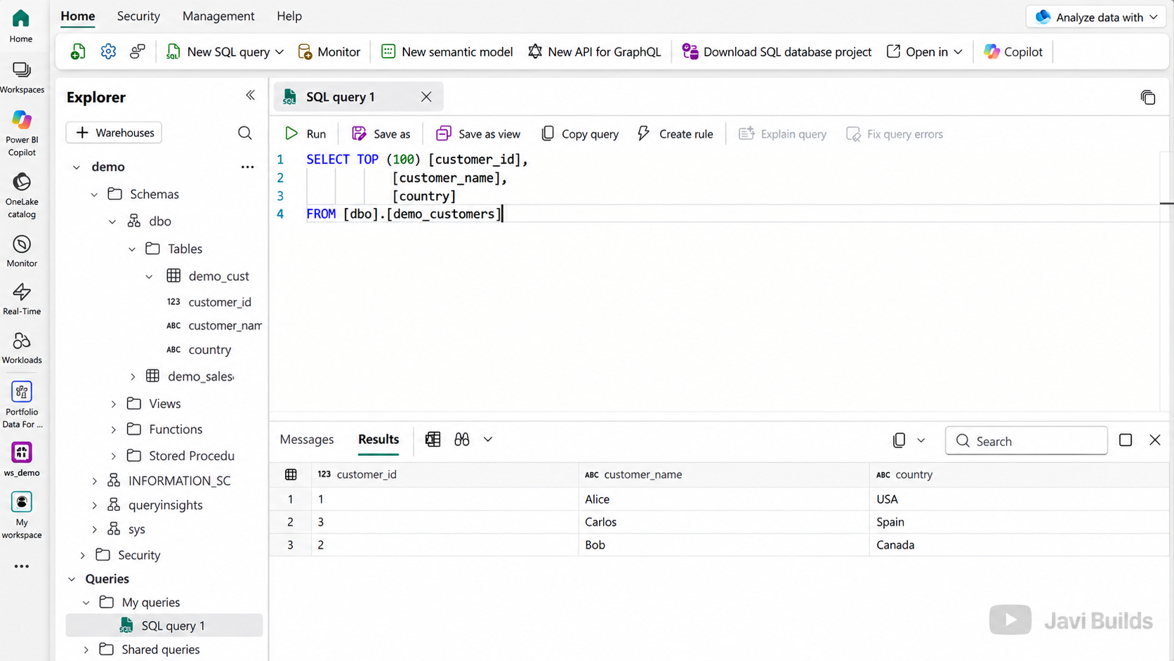
The Lakehouse SQL analytics endpoint lets SQL users query the same Lakehouse tables without opening a notebook.
This is a different experience from the %%sql cells in Step 7. Spark SQL runs through Spark inside the notebook; the SQL analytics endpoint provides a SQL query experience outside the notebook, over the same Lakehouse tables.
| Spark SQL in Notebook | SQL analytics endpoint |
|---|---|
| Runs through Spark | SQL endpoint experience |
| Used inside notebooks | Used from the SQL query editor and SQL tools |
| Good for mixed PySpark + SQL workflows | Good for SQL-oriented querying |
| Works through Spark execution | Exposes Lakehouse tables through SQL |
| Can write Delta tables | Read-only for Lakehouse table data |
Both read the same Delta tables in OneLake; nothing is copied between them. Tables the notebook creates, such as demo_sales_by_country in Step 9, become queryable from the endpoint as well, typically after a short metadata sync.
Step 12: Parameterize the notebook
Avoid hardcoded run values:
process_date = "2026-10-09"
tenant_id = 42
Fabric notebooks support a designated parameter cell.
A parameter cell can define defaults such as:
process_date = "2026-10-09"
tenant_id = 0
full_reload = FalseWhen a Fabric pipeline invokes the notebook, the Notebook activity can provide parameter values.
Notebook parameters support simple types such as string, int, float, and bool.
A useful shape is:
- 1Parameters
- 2Validate parameters
- 3Resolve configuration
- 4Execute transformation
- 5Write result
Step 13: Run the notebook from a Fabric pipeline
Create a Fabric Data Factory pipeline and add a Notebook activity. The pipeline owns scheduling, retries and branching while the notebook owns the transformation; choosing between pipelines, notebooks, Dataflow Gen2 and Copy jobs explains that split.
The pipeline can select the notebook and pass base parameters.
- Pipeline
- Notebook activity
- base parametersnb_transform_sales
- process_date
- tenant_id
The pipeline should usually own schedules, dependencies, retries, sequencing, and high-level execution state.
The notebook should usually own transformation logic, validation, data-quality checks, and writes.
Step 14: Add execution logging
A production notebook should let you answer:
Which run failed?
Which tenant?
Which process date?
When did it start?
When did it end?
How many rows were read?
How many were written?
What error occurred?
At minimum, establish a run context:
from datetime import datetime, timezone
import uuid

run_id = str(uuid.uuid4())
started_at = datetime.now(timezone.utc)

print(f"run_id={run_id}")
print(f"tenant_id={tenant_id}")
print(f"process_date={process_date}")
print(f"started_at={started_at.isoformat()}")For a real platform, persist run information to an execution-log table.
Useful fields often include:
run_id
parent_run_id
pipeline_name
notebook_name
tenant_id
process_date
status
started_at
ended_at
rows_read
rows_written
rows_rejected
error_code
error_message
Step 15: Fail deliberately when validation fails
A dangerous notebook detects a problem and continues:
if invalid_count > 0:
    print("Warning: invalid rows found")
If the output should not be trusted, fail explicitly:
if invalid_count > 0:
    raise ValueError(
        f"Validation failed: {invalid_count} invalid records found."
)That allows the orchestration layer to detect failure.
Step 16: Think about retry safety
If a pipeline retries your notebook, what happens?
A production notebook should not duplicate data because the first attempt wrote successfully before the activity failed.
Typical patterns include:
- stable business keys;
- Delta
MERGE; - partition replacement;
- idempotent append;
- processed-file tracking;
- watermark/checkpoint state.
The principle is:
A pipeline retry should not corrupt the destination.
Incremental Loads in Microsoft Fabric walks through a concrete failure, a notebook that commits Silver but dies before recording its watermark, and shows why the rerun stays safe.
Step 17: Source-control the notebook
Fabric notebooks support Git integration as part of Fabric lifecycle management.
Source control gives you:
- version history;
- branches;
- code review;
- visibility into changes;
- a path for promotion across environments.
A healthier model than editing directly in production is:
- Developer change
- Git branch
- Review
- DEV
- validationTEST / QA
- PROD
Your exact deployment mechanism can use Fabric Git integration, deployment pipelines, or CI/CD around Fabric APIs.
Step 18: Separate code from environment configuration
A notebook that contains workspace IDs, Lakehouse IDs, production endpoints, or secrets throughout its cells becomes difficult to promote.
Prefer environment-specific configuration outside the core transformation logic.
This becomes especially important when moving notebooks across:
DEV
QA
PROD
Step 19: Understand what Git does and does not deploy
Source control and deployment manage supported item metadata and code, not your business data itself.
A useful separation is:
Git
→ definitions / code / metadata

OneLake
→ actual data
Treat data migration and application deployment as related but separate concerns.
Step 20: Monitor notebook execution
A notebook is not finished when it succeeds once.
Track at least:
- duration;
- success/failure;
- row counts;
- input size;
- output size;
- retries;
- rejected records;
- repeated slowdowns.
A notebook that normally finishes in 4 minutes and suddenly takes 25 minutes may still technically succeed, but operationally it deserves investigation.
Step 21: Performance basics
Start with:
Where is the time actually going?
Possibilities include:
Spark session startup
data read
shuffle
join
serialization
write
small files
source latency
orchestration wait
Do not optimize Python syntax when the workload spends most of its time shuffling data in Spark.
Avoid unnecessary actions
Actions trigger execution:
df.count()
display(df)
df.collect()Use them deliberately.
Avoid large driver collections
rows = df.collect()can overwhelm the driver for large dataframes.
Watch joins
Before joining large datasets, understand:
- row counts;
- key cardinality;
- skew;
- duplicate keys;
- expected output cardinality.
Step 22: Keep notebook cells production-friendly
A good structure is:
1. Parameters
2. Imports
3. Configuration
4. Run context / logging
5. Read
6. Validate input
7. Transform
8. Validate output
9. Write
10. Final metrics
Production execution should not depend on manually running cells in a hidden order.
Step 23: Avoid hidden notebook state
A notebook can appear to work because a variable was created in a cell executed earlier.
Before considering it ready, test:
fresh session
→ Run all
→ success
If that fails, the notebook is not reproducible yet.
Step 24: Treat the notebook as a component
One notebook should not necessarily own ingestion, all transformations, orchestration, logging, notifications, and serving.
A cleaner boundary might be:
Pipeline
├── Copy raw data
├── Notebook: validate + standardize
├── Notebook: business transformation
├── Data-quality activity
└── Publish / notify
The boundary should reflect operational responsibilities.
Production-ready checklist
Data
- Is the input contract explicit?
- Are important keys validated?
- Are duplicates handled?
- Are invalid records accounted for?
Repeatability
- Does it run from a fresh session?
- Is it safe to retry?
- Are writes idempotent?
Configuration
- Are environment-specific values externalized?
- Are run values parameters rather than hardcoded?
Operations
- Does every run have an identity?
- Are start/end/status recorded?
- Are row counts captured?
- Does a critical validation issue fail the activity?
Performance
- Have large joins been checked?
- Are unnecessary Spark actions removed?
- Is driver collection avoided?
- Is the write strategy appropriate?
Lifecycle
- Is the notebook in source control?
- Can it move through DEV/TEST/PROD?
- Are dependent Lakehouses and environments understood?
From first notebook to production
- 1Notebook works interactively
- 2Notebook runs from a clean session
- 3Inputs and outputs are validated
- 4Parameters replace hardcoded values
- 5Writes become retry-safe
- 6Pipeline owns orchestration
- 7Execution is logged
- 8Git owns change history
- 9Deployment promotes across environments
- 10Production monitoring measures behavior
That is the difference between using a notebook and engineering a notebook workload.
Final thoughts
Microsoft Fabric makes it easy to create a notebook, connect it to a Lakehouse, and start transforming data.
But the engineering work starts after the first successful run.
A production notebook needs clear dependencies, parameters, validation, retry-safe writes, execution logging, source control, deployment discipline, and monitoring.
The goal is not to remove the flexibility that makes notebooks useful.
The goal is to keep that flexibility while adding enough structure that the notebook can be trusted in production.
Official Microsoft references
- Develop, execute, and manage Fabric notebooks: https://learn.microsoft.com/en-us/fabric/data-engineering/author-execute-notebook
- Explore Lakehouse data with a notebook: https://learn.microsoft.com/fabric/data-engineering/lakehouse-notebook-explore
- Load data into a Lakehouse with a notebook: https://learn.microsoft.com/en-us/fabric/data-engineering/lakehouse-notebook-load-data
- Lakehouse tutorial: https://learn.microsoft.com/en-us/fabric/data-engineering/tutorial-build-lakehouse
- Notebook activity in Fabric Data Factory: https://learn.microsoft.com/en-us/fabric/data-factory/notebook-activity
- Notebook source control and deployment: https://learn.microsoft.com/en-us/fabric/data-engineering/notebook-source-control-deployment
Was this helpful?
What could be better?
Thanks — that helps me improve Javi Builds.
Continue learning
- Cheat sheetMonitor Fabric Pipelines and NotebooksMonitor Microsoft Fabric pipelines and notebooks using Monitoring hub, Workspace Monitoring, Spark monitoring, KQL, alerts, and capacity telemetry so failures and performance regressions become observable.Open cheat sheet
- ResourceFabric Notebook Performance ChecklistA practical pre-run, read, transform, write and orchestration checklist for faster and more reliable Microsoft Fabric notebooks.View resource
What should I build next?
I'm building Javi Builds around practical problems data engineers actually face. Tell me what you'd like to see next.
Stay in the loop
Get the Javi Builds updates you actually care about.
Check your inbox
I sent you a confirmation link. Your subscription will be active after you confirm it.